JUMP TO TOPIC
Mean median mode – Explanation & Examples
 The definition of mean, median, and mode is:
“Mean, median, and mode are different measures of center in numerical data”.
In this topic, we will discuss the mean, median, and mode from the following aspects:
- What is mean, median, and mode in statistics?
- How to find the mean, median, and mode?
- The difference between mean and median.
- Practical questions.
- Answers.
What is mean, median, and mode in statistics?
The mean, median, and mode are different measures of the central tendency (central location) of numerical data.
A measure of central tendency is a single value that tries to describe numerical data by identifying the central position of that data.
As such, measures of central tendency are also called summary statistics because they try to summarize a numerical dataset with a single number.
The mean, median and mode are all measures of central tendency, but under certain conditions, some measures of central tendency become more suitable to use than others.
How to find the mean, median, and mode?
The mean
The mean of a set of numbers can be found by summing the numbers and dividing by their count.
The mean has one main disadvantage, it is sensitive to the effect of outliers. The outliers are values that are unusual compared to the rest of the data by being smaller or larger in numerical value.
With more outliers in your data, the mean loses its ability to provide the central location for the data because the outlier values drag the mean away from the central position.
Example 1
The following is the age in years of 20 individuals:
25 25 26 36 39 40 40 44 44 44 45 47 48 51 52 52 52 53 67 77.
The mean of this data is:
(25+25+26+36+39+40+40+44+44+44+45+47+48+51+52+52+52+53+67+77)/20 = 907/20 = 45.35 years.
If we only change the last value to a more larger (outlier) value, 118, the mean will be:
(25+25+26+36+39+40+40+44+44+44+45+47+48+51+52+52+52+53+67+118)/20 = 948/20 = 47.4 years.
If we change the last 5 values to a more larger (outlier) value, 118, the mean will be:
(25+25+26+36+39+40+40+44+44+44+45+47+48+51+52+118+118+118+118+118)/20 = 1196/20 = 59.8 years.
The mean is dragged to the side of large values away from the central position.
In the last case where the mean equals 59.8 years, the mean is no longer a reliable summary statistic for the data center, because the majority of the data is in the range 25-52 years.
If we only change the first value to a more smaller (outlier) value, 1, the mean will be:
(1+25+26+36+39+40+40+44+44+44+45+47+48+51+52+52+52+53+67+77)/20 = 883/20 = 44.15 years.
If we change the first 5 values to a more smaller (outlier) value, 1, the mean will be:
(1+1+1+1+1+40+40+44+44+44+45+47+48+51+52+52+52+53+67+77)/20 = 761/20 = 38.05 years.
The mean is dragged to the side of small values away from the central position and is no longer a reliable summary statistic for the data center because the majority of the data is in the range 40-77 years.
Example 2
The following is the weight in kilograms of 15 individuals:
64.0 87.0 46.0 69.0 67.3 59.0 71.0 87.0 85.0 62.0 68.0 80.0 82.5 67.0 66.0.
The mean of this data is:
(64.0+87.0+46.0+69.0+67.3+59.0+71.0+87.0+85.0+62.0+68.0+80.0+82.5+67.0+66.0)/15 = 1060.8/15 = 70.72 kilograms.
If we only change the last value to a more larger (outlier) value, 130, the mean will be:
(64.0+87.0+46.0+69.0+67.3+59.0+71.0+87.0+85.0+62.0+68.0+80.0+82.5+67.0+130.0)/15 = 1124.8/15 = 74.99 kilograms.
If we change the last 5 values to a more larger (outlier) value, 130, the mean will be:
(64.0+87.0+46.0+69.0+67.3+59.0+71.0+87.0+85.0+62.0+130.0+130.0+130.0+130.0+ 130.0)/15 = 1347.3/15 = 89.82 kilograms.
The mean is dragged to the side of large values away from the central position.
If we only change the first value to a more smaller (outlier) value, 1, the mean will be:
(1+87.0+46.0+69.0+67.3+59.0+71.0+87.0+85.0+62.0+68.0+80.0+82.5+67.0+66.0)/15 = 997.8/15 = 66.52 kilograms.
If we only change the first 5 values to a more smaller (outlier) value, 1, the mean will be:
(1+1+1+1+1+59.0+71.0+87.0+85.0+62.0+68.0+80.0+82.5+67.0+66.0)/15 = 732.5/15 = 48.83 kilograms.
The mean is dragged to the side of small values away from the central position.
The median
The median is the value that halves a set of data values equally. In other words, it is the middle value of a data set.
The median always retains its position and is not influenced by the outlier values.
If we have an odd set of numbers, we sort them first, and then the median is the middle number with an equal amount of numbers above and below it.
If we have an even set of numbers, the numbers are sorted and the middle two numbers are selected. Then, these two numbers are added together and divided by two to get the median.
Example 1 of an even list of numbers
The following is the age in years of 20 individuals.
We have 20 age values which is an even number.
25 25 26 36 39 40 40 44 44 44 45 47 48 51 52 52 52 53 67 77.
- The data is already sorted from lower to higher values.
- We pick the middle pair:
25 25 26 36 39 40 40 44 44 44 45 47 48 51 52 52 52 53 67 77.
The middle pair is (44,45) because it has 9 numbers before it (25,25,26, 36,39, 40, 40, 44, 44) and 9 numbers after it (47, 48, 51, 52, 52, 52, 53, 67, 77).
- We sum the middle pair and divide by 2 to get the median.
The median = (44+45)/2 = 44.5 years, while the mean = 45.35 years.
If we only change the last value to a more larger (outlier) value, 118, the median will be:
25 25 26 36 39 40 40 44 44 44 45 47 48 51 52 52 52 53 67 118.
The middle pair is (44,45) because it still has 9 numbers before it (25,25,26,36,39, 40, 40, 44, 44) and 9 numbers after it (47, 48, 51, 52, 52, 52, 53, 67, 118).
We sum the middle pair and divide by 2 to get the median.
The median = (44+45)/2 = 44.5 years also.
The mean = 47.4 years.
If we change the last 5 values to a more larger (outlier) value, 118, the median will be:
25 25 26 36 39 40 40 44 44 44 45 47 48 51 52 118 118 118 118 118.
The middle pair is also (44,45), and the median = (44+45)/2 = 44.5 years also.
The mean = 59.8 years.
If we only change the first value to a smaller (outlier) value, 1, the median will be:
1 25 26 36 39 40 40 44 44 44 45 47 48 51 52 52 52 53 67 77.
The middle pair is also (44,45), and the median = 44.5 years also, while the mean = 44.15 years.
If we change the first 5 values to a more smaller (outlier) value, 1, the median will be:
1 1 1 1 1 40 40 44 44 44 45 47 48 51 52 52 52 53 67 77.
The middle pair is also (44,45), and the median = 44.5 years also, while the mean = 38.05 years.
The presence of outlier small or large values has not dragged the median from the central position.
The median is still a reliable summary statistic of the central position of this data.
Example 2 of an odd list of numbers
The following is the weight in kilograms of 15 individuals.
We have 15 weight values which is an odd number.
64.0 87.0 46.0 69.0 67.3 59.0 71.0 87.0 85.0 62.0 68.0 80.0 82.5 67.0 66.0.
- We sort the data from lower to higher values.
46.0 59.0 62.0 64.0 66.0 67.0 67.3 68.0 69.0 71.0 80.0 82.5 85.0 87.0 87.0.
- We pick the middle value:
46.0 59.0 62.0 64.0 66.0 67.0 67.3 68.0 69.0 71.0 80.0 82.5 85.0 87.0 87.0.
The middle value is (68.0) because it has 7 numbers before it (46.0, 59.0, 62.0, 64.0, 66.0, 67.0, 67.3) and 7 numbers after it (69.0, 71.0, 80.0, 82.5, 85.0, 87.0, 87.0).
- The picked middle value is the median.
The median = 68.0 kilograms.
Note that the mean of this data is 70.72 kilograms.
If we only change the last value to a more larger (outlier) value, 130, the median will be:
46.0 59.0 62.0 64.0 66.0 67.0 67.3 68.0 69.0 71.0 80.0 82.5 85.0 87.0 130.0.
The median is 68.0 kilograms also, while the mean = 74.99 kilograms.
If we change the last 5 values to a more larger (outlier) value, 130, the median will be:
46.0 59.0 62.0 64.0 66.0 67.0 67.3 68.0 69.0 71.0 130.0 130.0 130.0 130.0 130.0.
The median is 68.0 kilograms also, while the mean = 89.82 kilograms.
If we only change the first value to a more smaller (outlier) value, 1, the median will be:
1 59.0 62.0 64.0 66.0 67.0 67.3 68.0 69.0 71.0 80.0 82.5 85.0 87.0 87.0.
The median is 68.0 kilograms also, while the mean = 66.52 kilograms.
If we only change the first 5 values to a more smaller (outlier) value, 1, the median will be:
1 1 1 1 1 67.0 67.3 68.0 69.0 71.0 80.0 82.5 85.0 87.0 87.0.
The median is 68.0 kilograms also, while the mean = 48.83 kilograms.
The mean is dragged to the side of large or small values away from the central position. On the other hand, the median retains its central position and is not affected by these outliers.
The mode
The mode is the value that appears most frequently in a set of data values. In other words, the mode is the number that has the highest number of occurrences.
One of the problems with the mode is that it may not be unique, so we may get stuck as to which mode value best describes the central tendency of the data.
The mode of a set of numbers can be found graphically using a bar graph or by using a frequency table.
Example 1
The following is the age in years of 20 individuals:
25 25 26 36 39 40 40 44 44 44 45 47 48 51 52 52 52 53 67 77.
- Graphical plot
We can plot this data as a bar graph where we plot the data values on a certain axis against their frequency on the other axis.
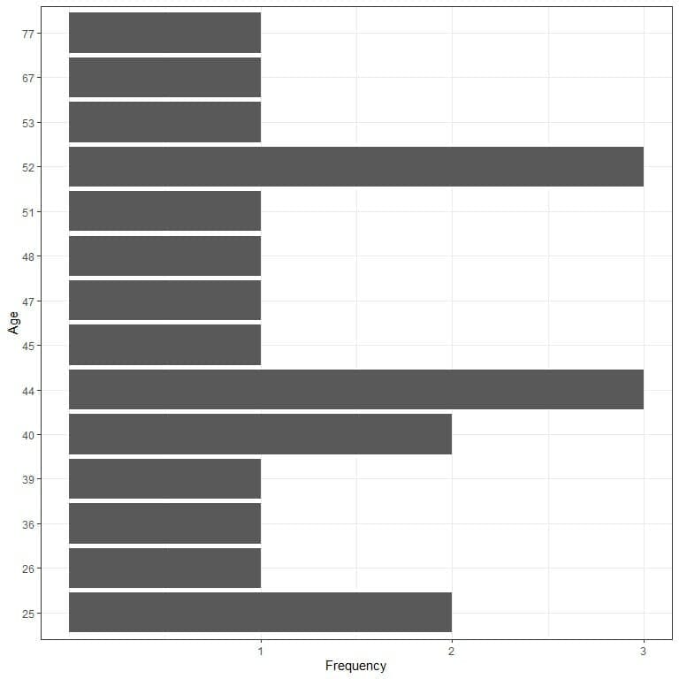
We see that all data values have occurred only once except:
- Values 25 and 40 occurred twice.
- Values 44 and 52 which occurred 3 times.
The mode of this data is 44 and 52 years because both numbers have the maximum occurrences in this data (3 times).
This is an example of Bimodal data.
- Frequency table
Where we tabulate the data values in one column and their frequency in another column.
Age | frequency |
25 | 2 |
26 | 1 |
36 | 1 |
39 | 1 |
40 | 2 |
44 | 3 |
45 | 1 |
47 | 1 |
48 | 1 |
51 | 1 |
52 | 3 |
53 | 1 |
67 | 1 |
77 | 1 |
We see also that both 44 and 52 have the maximum number of occurrences in this data so the mode is 44 and 52.
Now, we get stuck as to which mode value best describes the center of this data.
Example 2
The following is the weight in kilograms of 15 individuals:
64.0 87.0 46.0 69.0 67.3 59.0 71.0 87.0 85.0 62.0 68.0 80.0 82.5 67.0 66.0.
- Graphical plot

We see that all data values have occurred only once except:
- Value 87 which occurred twice.
The mode of this data is 87 kilograms because this number has the maximum occurrences in this data (2 times).
This is an example of Unimodal data.
- Frequency table
Weight | frequency |
46 | 1 |
59 | 1 |
62 | 1 |
64 | 1 |
66 | 1 |
67 | 1 |
67.3 | 1 |
68 | 1 |
69 | 1 |
71 | 1 |
80 | 1 |
82.5 | 1 |
85 | 1 |
87 | 2 |
We see also that 87 has the maximum number of occurrences in this data so the mode is 87.
Normally, the mode is used for categorical data where we wish to know which is the most common category.
Example 3
The following is the marital status of 50 individuals:
id | marital status |
1 | Never married |
2 | Divorced |
3 | Widowed |
4 | Never married |
5 | Divorced |
6 | Married |
7 | Never married |
8 | Divorced |
9 | Married |
10 | Married |
11 | Married |
12 | Married |
13 | Married |
14 | Married |
15 | Divorced |
16 | Married |
17 | Widowed |
18 | Never married |
19 | Married |
20 | Married |
21 | Married |
22 | Married |
23 | Never married |
24 | Widowed |
25 | Widowed |
26 | Widowed |
27 | Widowed |
28 | Widowed |
29 | Divorced |
30 | Widowed |
31 | Widowed |
32 | Married |
33 | Married |
34 | Never married |
35 | Married |
36 | Never married |
37 | Never married |
38 | Never married |
39 | Never married |
40 | Never married |
41 | Married |
42 | Married |
43 | Divorced |
44 | Never married |
45 | Never married |
46 | Never married |
47 | Married |
48 | Married |
49 | Married |
50 | Married |
- Graphical plot
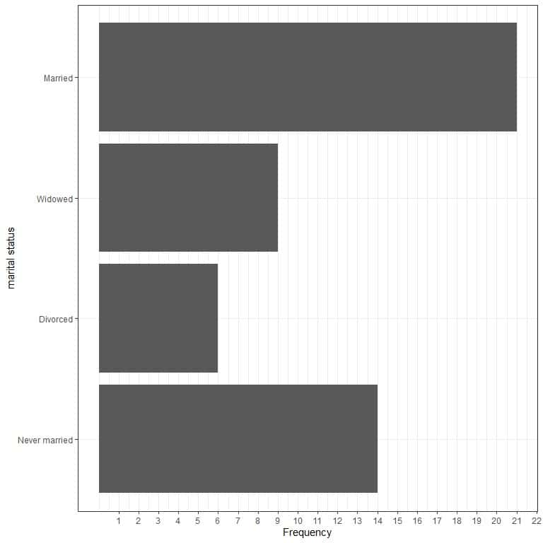
- Frequency table
marital status | frequency |
Never married | 14 |
Divorced | 6 |
Widowed | 9 |
Married | 21 |
The mode of this data is married because the married status has the maximum occurrences in this data (21 times).
This is an example of Unimodal data.
The difference between the mean and the median
If you have a normally distributed sample, you can use the mean or the median as a measure of central tendency or central location.
In a normal distribution, data is symmetrically distributed around a central region. Values closer to the central region are more frequent than values far from the central region.
The mean and the median are nearly the same in a normal distribution.
You can see that your sample is normally distributed by plotting a histogram of your data where we use a bin frequency table to plot the data bins on a certain axis against their frequency on the other axis.
The bin frequency table groups values into equal-sized bins and each bin includes a range of values.
Example 1 of normally distributed data
The following bin frequency table lists the diastolic blood pressure of 2280 persons.
range | frequency |
40 – 45 | 1 |
45 – 50 | 4 |
50 – 55 | 12 |
55 – 60 | 59 |
60 – 65 | 103 |
65 – 70 | 288 |
70 – 75 | 300 |
75 – 80 | 526 |
80 – 85 | 343 |
85 – 90 | 329 |
90 – 95 | 157 |
95 – 100 | 97 |
100 – 105 | 27 |
105 – 110 | 25 |
110 – 115 | 5 |
115 – 120 | 2 |
120 – 125 | 2 |
The bin 40-45 includes all values from 40 to 45. The frequency is 1 meaning that one person of the 2280 persons has a diastolic blood pressure in this range.
The next bin 45-50 includes all values larger than 45 till 50. The frequency is 4 meaning that 4 persons of the 2280 persons have diastolic blood pressure in this range.
We see that the most frequent bin is bin 75-80 with 526 frequency. This means that 526 persons of the 2280 persons have diastolic blood pressure in this range.
If we sum these frequencies, we will get the number 2280.
If we use this table to plot a histogram.
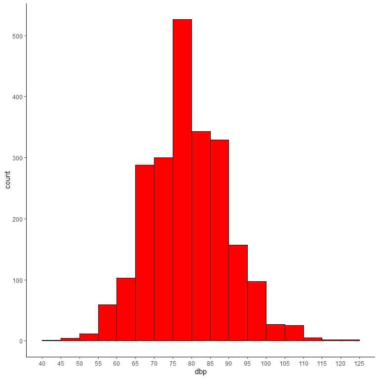
We see that the most frequent bin is bin 75-80 with more than 500 counts or frequency.
We can add different lines that correspond to the single values of mean and median.
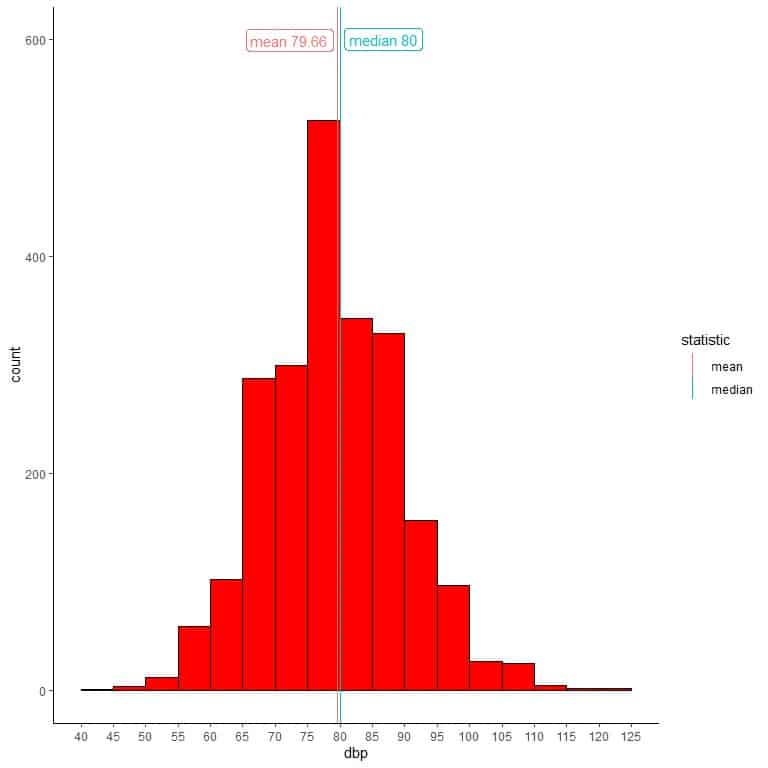
We see that the mean and the median are nearly equal to 80.
Most of the data cluster in the center providing a normally distributed shape.
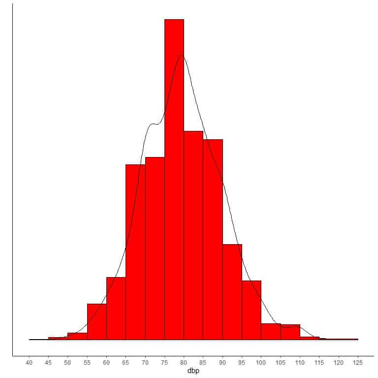
If we overlay this histogram with a density curve to observe the data distribution, we get nearly the bell-shaped curve of a normal distribution.
In skewed distributions, more values are clustered on one side of the center than the other, and the mean and the median differ from each other.
In a positively skewed distribution (right-skewed), there’s a cluster of lower values on the left side of the numerical scale and a rare larger value on the right side.
In a negatively skewed distribution (left-skewed), there’s a cluster of higher values on the right side of the numerical scale and a rare smaller values on the left side.
In these cases, the mean is no longer a suitable measurement of central tendency and we only rely on the median.
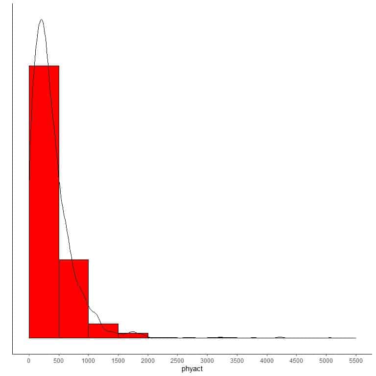
Example 2 of right-skewed data
The following bin frequency table lists the physical activity (Kcal/week) for 2206 persons.
range | frequency |
0 – 500 | 1615 |
500 – 1000 | 465 |
1000 – 1500 | 85 |
1500 – 2000 | 29 |
2000 – 2500 | 3 |
2500 – 3000 | 2 |
3000 – 3500 | 3 |
3500 – 4000 | 1 |
4000 – 4500 | 2 |
4500 – 5000 | 0 |
5000 – 5500 | 1 |
We see that the most frequent bin is bin 0-500 with 1615 occurrences. This is the main cluster of data which is on the extreme left side (small side) of the numerical scale.
Larger bins (with physical activity of more than 2000) have very low frequency and never exceed 5.
If we use this table to plot a histogram.
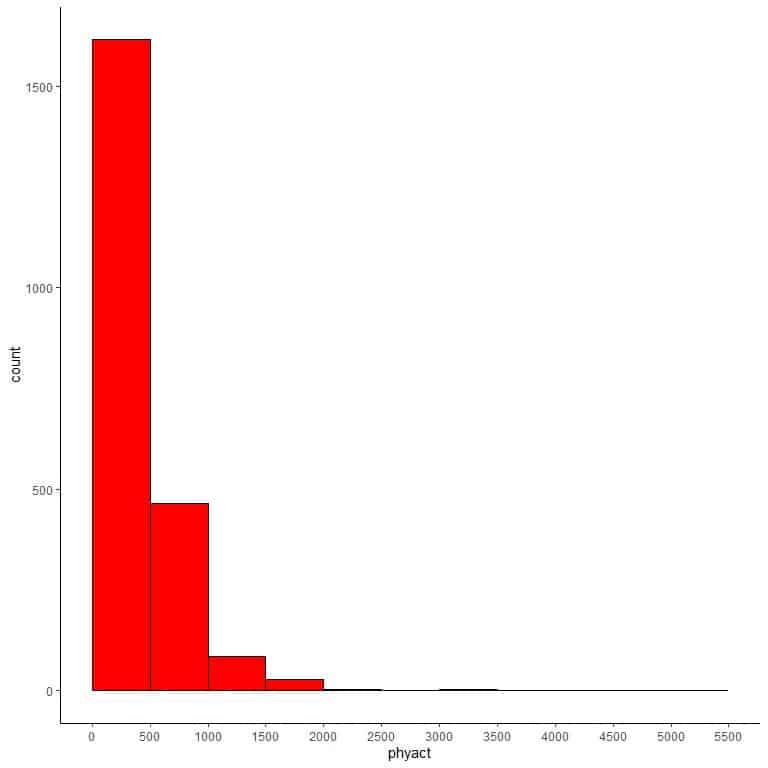
We see that the main cluster of data is on the left side of the numerical scale and rare large values on the right side.
We can add different lines for the single values of mean or median.
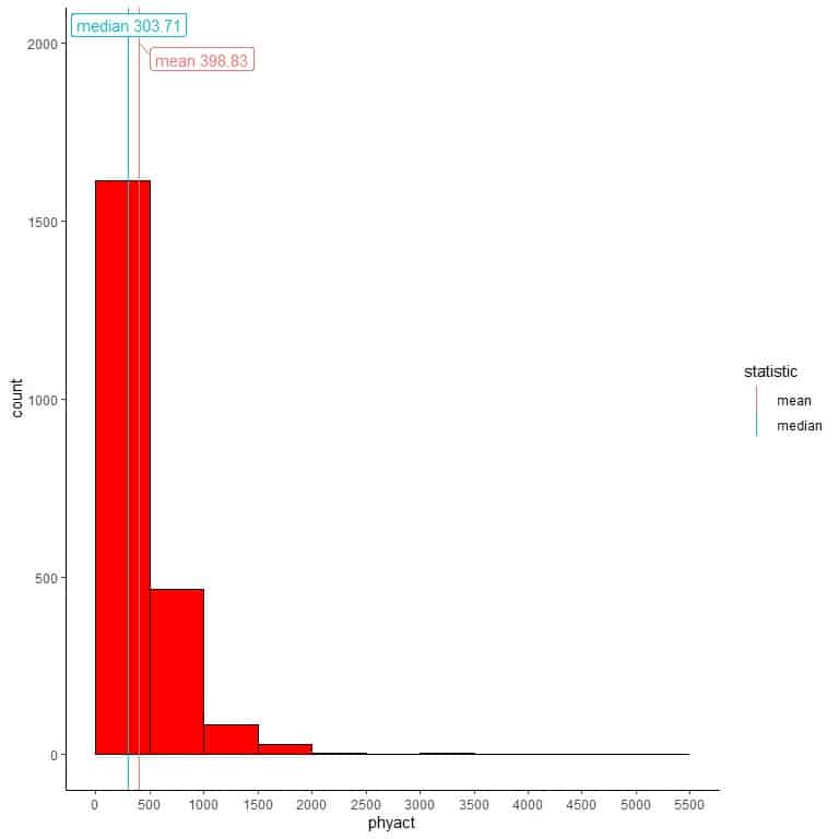
We see that the median=303.71 is far less than the mean = 398.83.
If we overlay this histogram with a density curve to observe the data distribution, we get a peak at the left side and a long tail at the right side, so this distribution is called “right-skewed distribution”.
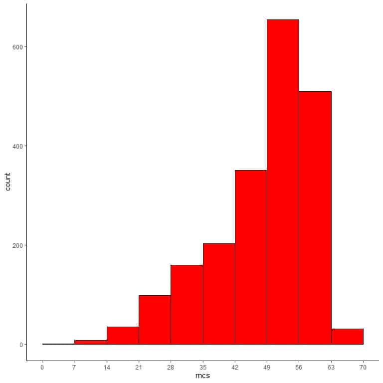
Example 3 of left-skewed data
The following bin frequency table lists the mental component for 2054 persons.
range | frequency |
0 – 7 | 1 |
7 – 14 | 8 |
14 – 21 | 36 |
21 – 28 | 99 |
28 – 35 | 160 |
35 – 42 | 203 |
42 – 49 | 351 |
49 – 56 | 654 |
56 – 63 | 510 |
63 – 70 | 32 |
We see that the most frequent bin is bin 49-56 with 654 occurrences. This is the main cluster of data which is on the extreme right side (large side) of the numerical scale.
Smaller value bins have a much lower frequency.
If we use this table to plot a histogram.
We can add different lines for the values of the mean and the median.
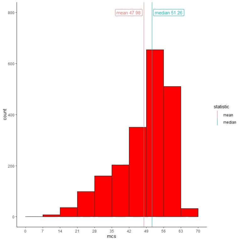
We see that the median=51.26 is far larger than the mean = 47.98.
Most of the data cluster on the right side of the numerical scale with rare small values on the left side.
If we overlay this histogram with a density curve to observe the data distribution, we get a peak at the right side and a long tail at the left side so named “left-skewed distribution”.

In conclusion
We can assess the distribution of numerical data by looking at the histograms or by looking at the mean and median:
- If the mean nearly equals the median, we can conclude that our data is normally distributed. We can use either mean or median as a summary statistic for the data center.
- If the mean is far larger than the median, we can conclude that our data is right-skewed (positively skewed). We should rely on the median as a summary statistic for the data center.
- If the mean is far less than the median, we can conclude that our data is left-skewed (negatively skewed). We should rely on the median as a summary statistic for the data center.
Practical questions
- The following table is the mean and median age for 3129 Black persons and 16395 White persons.
race | mean age | median age |
Black | 43.89727 | 42 |
White | 48.72493 | 48 |
Comment on the age distribution for Whites and Blacks in this data.
- The following table is the mean and median age for 1101 males and 1193 females.
sex | mean age | median age |
Male | 54.78474 | 54 |
Female | 54.69153 | 55 |
Comment on the age distribution for males and females in this data.
- The following table is the mean and median weight for 723 hypertensive persons and 1563 non-hypertensive persons.
hypertension | mean weight | median weight |
Yes | 76.90098 | 77 |
No | 71.81358 | 71 |
Which group has a higher mean? Which group has a higher median?
- The following table is the mean, median, and mode of physical activity for 709 persons with hypercholesterolemia and 1564 persons without hypercholesterolemia.
hypercholesterolemia | mean activity | median activity | mode activity |
Yes | 385 | 304 | 155 |
No | 406 | 303 | 156 |
Which group has a higher mean? Which group has a higher median? which group has a higher mode?
Comment on the physical activity distribution for both groups.
- The following table is the mean and median pressure for 3091 hurricane storms, 2545 tropical depression storms, and 4374 tropical storms.
status | mean pressure | median pressure |
hurricane | 969 | 973 |
tropical depression | 1008 | 1008 |
tropical storm | 999 | 1000 |
Which group has typical normally distributed pressure?
Which group has more skewed pressure and of what type (right-skewed or left-skewed)?
Answers
- The mean and median age for White persons is nearly equal meaning that the age in White persons is normally distributed. The mean age is larger than the median age for Black persons. This means that the age in Black persons is right-skewed.
- The mean and median age for males is nearly equal. This is also observed for females. This means that the age in males or females is normally distributed.
- The hypertensive persons have higher mean weight and higher median weight than the non-hypertensive persons.
- Persons without hypercholesterolemia have higher mean activity and higher mode activity than persons with hypercholesterolemia. Persons with hypercholesterolemia have higher median activity than persons without hypercholesterolemia. In both groups, the mean is larger than the median which means that the physical activity in both groups is right-skewed.
- The “tropical depression” has typical normal distribution because the mean = median = 1008. The “hurricane” group has more left-skewed pressure distribution because the mean is far less than the median.