Frequency table – Explanation & Examples
 The definition of frequency table is:
“The frequency table is a table that shows the frequency of different items in your data”.
In this topic, we will discuss the frequency table from the following aspects:
- What is a frequency table?
- How to do a frequency table?
- Practical questions.
- Answers.
What is a frequency table?
A frequency table is a table that lists the number of occurrences (frequency) of different items in your data.
The different items can be categorical data or numeric data.
Example 1 of categorical data
The following are the smoking habits of 10 participants from a certain survey. Each individual chooses his smoking habit as “Never smoker”, “Current or former < 1y”, for current or former smokers who quit smoking for less than 1 year, or “Former >= 1y” for former smokers who quit smoking for more than or equal to 1 year.
participant | Smoking habit |
1 | Never smoker |
2 | Never smoker |
3 | Current or former < 1y |
4 | Never smoker |
5 | Current or former < 1y |
6 | Never smoker |
7 | Never smoker |
8 | Former >= 1y |
9 | Former >= 1y |
10 | Former >= 1y |
We can list the occurrences of different smoking habits in the following frequency table.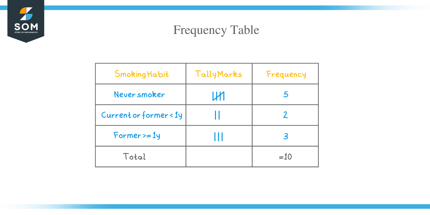
Smoking habit | frequency |
Never smoker | 5 |
Current or former < 1y | 2 |
Former >= 1y | 3 |
We see that the most frequent smoking habit is “Never smoker” with 5 occurrences and the least frequent smoking habit is “Current or former < 1y” smoking habit with only 2 occurrences.
Example 2 of categorical data
The following is the gender of 10 participants from a certain survey. Each individual chooses gender as Male or Female.
participant | Gender |
1 | Female |
2 | Female |
3 | Male |
4 | Female |
5 | Female |
6 | Female |
7 | Male |
8 | Female |
9 | Female |
10 | Male |
We can list the occurrences of the two genders in the following frequency table.
Gender | frequency |
Male | 3 |
Female | 7 |
We see that the most frequent gender is “Female” with 7 occurrences and “Male” has the remaining 3 occurrences.
Example 3 of numerical data
The following is the number of cylinders for 32 different car models in 1973-1974.
Model | Number of cylinders |
Mazda RX4 | 6 |
Mazda RX4 Wag | 6 |
Datsun 710 | 4 |
Hornet 4 Drive | 6 |
Hornet Sportabout | 8 |
Valiant | 6 |
Duster 360 | 8 |
Merc 240D | 4 |
Merc 230 | 4 |
Merc 280 | 6 |
Merc 280C | 6 |
Merc 450SE | 8 |
Merc 450SL | 8 |
Merc 450SLC | 8 |
Cadillac Fleetwood | 8 |
Lincoln Continental | 8 |
Chrysler Imperial | 8 |
Fiat 128 | 4 |
Honda Civic | 4 |
Toyota Corolla | 4 |
Toyota Corona | 4 |
Dodge Challenger | 8 |
AMC Javelin | 8 |
Camaro Z28 | 8 |
Pontiac Firebird | 8 |
Fiat X1-9 | 4 |
Porsche 914-2 | 4 |
Lotus Europa | 4 |
Ford Pantera L | 8 |
Ferrari Dino | 6 |
Maserati Bora | 8 |
Volvo 142E | 4 |
We can list the occurrences of the number of cylinders in the following frequency table.
Number of cylinders | frequency |
4 | 11 |
6 | 7 |
8 | 14 |
We see that the most frequent number of cylinders is 8 with 14 occurrences or 14 different cars have this number of cylinders. The least frequent number is 6 with only 6 cars having this number.
Example 4 of numerical data
The following are the weights of 39 participants (in Kg) from a certain survey.
participant | Weight |
1 | 64.0 |
2 | 67.0 |
3 | 70.0 |
4 | 68.0 |
5 | 43.5 |
6 | 79.2 |
7 | 45.8 |
8 | 53.0 |
9 | 62.0 |
10 | 79.0 |
11 | 66.0 |
12 | 65.0 |
13 | 60.0 |
14 | 69.0 |
15 | 69.0 |
16 | 88.0 |
17 | 76.0 |
18 | 69.0 |
19 | 80.0 |
20 | 77.0 |
21 | 63.4 |
22 | 72.0 |
23 | 65.5 |
24 | 75.0 |
25 | 84.0 |
26 | 76.0 |
27 | 55.0 |
28 | 64.0 |
29 | 80.0 |
30 | 95.5 |
31 | 58.0 |
32 | 84.5 |
33 | 65.0 |
34 | 70.0 |
35 | 50.4 |
36 | 68.0 |
37 | 94.0 |
38 | 88.0 |
39 | 68.0 |
We can list the occurrences of these weights in the following frequency table.
Weight | frequency |
43.5 | 1 |
45.8 | 1 |
50.4 | 1 |
53 | 1 |
55 | 1 |
58 | 1 |
60 | 1 |
62 | 1 |
63.4 | 1 |
64 | 2 |
65 | 2 |
65.5 | 1 |
66 | 1 |
67 | 1 |
68 | 3 |
69 | 3 |
70 | 2 |
72 | 1 |
75 | 1 |
76 | 2 |
77 | 1 |
79 | 1 |
79.2 | 1 |
80 | 2 |
84 | 1 |
84.5 | 1 |
88 | 2 |
94 | 1 |
95.5 | 1 |
We see that the frequency table is long and noninformative as we have many different weight values.
In that case, we use a bin frequency table. The bin frequency table groups values into equal-sized bins and each bin includes a range of values.
range | frequency | original values |
43.5 – 53.5 | 4 | 43.5, 45.8, 50.4, 53.0 |
53.5 – 63.5 | 5 | 55.0, 58.0, 60.0, 62.0, 63.4 |
63.5 – 73.5 | 16 | 64.0, 64.0, 65.0, 65.0, 65.5, 66.0, 67.0, 68.0, 68.0, 68.0, 69.0, 69.0, 69.0, 70.0, 70.0, 72.0 |
73.5 – 83.5 | 8 | 75.0, 76.0, 76.0, 77.0, 79.0, 79.2, 80.0, 80.0 |
83.5 – 93.5 | 4 | 84.0, 84.5, 88.0, 88.0 |
93.5 – 103.5 | 2 | 94.0, 95.5 |
Here we group the data or weights into 6 equal-sized bins. Each bin includes a range of certain values.
For example, the bin “43.5-53.5” includes weights from 43.5 to 53.5 Kg.
The bin “53.5-63.5” includes values larger than 53.5 Kg to 63.5 Kg and so on.
If you sum these frequencies, you will get 39 which is the total number of data.
How to do a frequency table?
Example 1 of categorical data
The following is the marital status of 20 participants from a certain survey.
participant | Marital status |
1 | Never married |
2 | Divorced |
3 | Widowed |
4 | Never married |
5 | Divorced |
6 | Married |
7 | Never married |
8 | Divorced |
9 | Married |
10 | Married |
11 | Married |
12 | Married |
13 | Married |
14 | Married |
15 | Divorced |
16 | Married |
17 | Widowed |
18 | Never married |
19 | Married |
20 | Married |
We can make a frequency table of this by following these steps:
- We draw a table of 3 columns. The first column carries the different categories of our data.
We see from the original data table that the marital status categories are Never married, Divorced, Widowed, and Married.
Marital status |
Never married |
Divorced |
Widowed |
Married |
- The second column contains the tally marks for each category.
When any category occurs, a tally mark is added to the chart in front of the value or category name. Every fifth tally is drawn vertically to make a collection of five.
The first value is Never married so we add a tally mark to the Never married row.
The second value is Divorced so we add a tally mark to the Divorced row.
The third value is Widowed so we add a tally mark to the Widowed row.
The fourth value is Never married so we add a (second) tally mark to the Never married row.
Marital status | Tally marks |
Never married | || |
Divorced | | |
Widowed | | |
Married |
We continue till we record all the 20 marital statuses as tally marks.
Marital status | Tally marks |
Never married | |||| |
Divorced | |||| |
Widowed | || |
Married | |||| |||| |
- The third column contains the frequency of each category.
Multiply the bundles of tallies by 5 and adding the individual tallies to obtain the frequency of each value or category.
For example, the Married marital status contains 2 bundles of 5 so the frequency = 2 X 5 = 10.
Marital status | Tally marks | Frequency |
Never married | |||| | 4 |
Divorced | |||| | 4 |
Widowed | || | 2 |
Married | |||| |||| | 10 |
Example 2 of numerical data with repeated values
The following is the number of forward gears for 32 different car models in 1973-1974.
Model | gear |
Mazda RX4 | 4 |
Mazda RX4 Wag | 4 |
Datsun 710 | 4 |
Hornet 4 Drive | 3 |
Hornet Sportabout | 3 |
Valiant | 3 |
Duster 360 | 3 |
Merc 240D | 4 |
Merc 230 | 4 |
Merc 280 | 4 |
Merc 280C | 4 |
Merc 450SE | 3 |
Merc 450SL | 3 |
Merc 450SLC | 3 |
Cadillac Fleetwood | 3 |
Lincoln Continental | 3 |
Chrysler Imperial | 3 |
Fiat 128 | 4 |
Honda Civic | 4 |
Toyota Corolla | 4 |
Toyota Corona | 3 |
Dodge Challenger | 3 |
AMC Javelin | 3 |
Camaro Z28 | 3 |
Pontiac Firebird | 3 |
Fiat X1-9 | 4 |
Porsche 914-2 | 5 |
Lotus Europa | 5 |
Ford Pantera L | 5 |
Ferrari Dino | 5 |
Maserati Bora | 5 |
Volvo 142E | 4 |
There are only 3 different numbers in this data, 3, 4, or 5 so we treat it as categorical data.
- We draw a table of 3 columns. The first column carries the different numbers of our data.
The second column contains the tally marks for each gear number.
The third column contains the frequency of each gear number.
gear |
3 |
4 |
5 |
- The second column contains the tally marks for each number.
When any gear number occurs, a tally mark is added to the chart in front of the value name. Every fifth tally is drawn vertically to make a collection of five.
The first value is 4 so we add a tally mark to the row of 4 gears.
The second value is 4 also, so we add a (second) tally mark to the row of 4 gears.
The third value is 4 also, so we add a (third) tally mark to the row of 4 gears.
The fourth value is 3 so we add a tally mark to the row of 3 gears.
gear | Tally marks |
3 | | |
4 | ||| |
5 |
We continue till we record all the 32 gear values as tally marks.
gear | Tally marks |
3 | |||| |||| |||| |
4 | |||| |||| || |
5 | |||| |
- The third column contains the frequency of each number of gears.
Multiply the bundles of tallies by 5 and adding the individual tallies to obtain the frequency of each value or category.
For example, the 3 gear contains 3 bundles of 5 so the frequency = 3 X 5 = 10.
the 4 gear contains 2 bundles of 5 and 2 individual tallies, so the frequency = (2 X 5)+2 = 12.
gear | Tally marks | Frequency |
3 | |||| |||| |||| | 15 |
4 | |||| |||| || | 12 |
5 | |||| | 5 |
Example 3 of numerical data with different values
The following is the age (in years) of 40 participants from a certain survey.
participant | Age |
1 | 26 |
2 | 48 |
3 | 67 |
4 | 39 |
5 | 25 |
6 | 25 |
7 | 36 |
8 | 44 |
9 | 44 |
10 | 47 |
11 | 53 |
12 | 52 |
13 | 52 |
14 | 51 |
15 | 52 |
16 | 40 |
17 | 77 |
18 | 44 |
19 | 40 |
20 | 45 |
21 | 48 |
22 | 49 |
23 | 19 |
24 | 54 |
25 | 82 |
26 | 83 |
27 | 89 |
28 | 88 |
29 | 72 |
30 | 82 |
31 | 89 |
32 | 34 |
33 | 55 |
34 | 37 |
35 | 22 |
36 | 33 |
37 | 37 |
38 | 43 |
39 | 29 |
40 | 57 |
If we list the occurrences of these age values with the normal frequency table.
Age | frequency |
19 | 1 |
22 | 1 |
25 | 2 |
26 | 1 |
29 | 1 |
33 | 1 |
34 | 1 |
36 | 1 |
37 | 2 |
39 | 1 |
40 | 2 |
43 | 1 |
44 | 3 |
45 | 1 |
47 | 1 |
48 | 2 |
49 | 1 |
51 | 1 |
52 | 3 |
53 | 1 |
54 | 1 |
55 | 1 |
57 | 1 |
67 | 1 |
72 | 1 |
77 | 1 |
82 | 2 |
83 | 1 |
88 | 1 |
89 | 2 |
We see that the frequency table is long and noninformative as we have many different age values.
In that case, we use a bin frequency table. The bin frequency table groups values into equal-sized bins and each bin includes a range of values.
Steps of a bin frequency table
- Determine the number of bins you need.
There are no hard rules about how many bins to pick, but there are some general guidelines:
- Pick between 5 and 20 classes.
- Make sure you have a few items in each bin. For example, if you have 40 data points, you can choose 5 bins (8 data points per category), but not 20 bins (which would give you only 2 data points per bin).
- Use the mathematical formula to choose classes.
The formula is log(observations)/ log(2). You would round up the answer to the next integer.
For our data, log(40)/log(2) = 5.3 will be rounded up to become 6.
- Sort the data and subtract the minimum data value from the maximum data value to get the data range.
The sorted data is:
19 22 25 25 26 29 33 34 36 37 37 39 40 40 43 44 44 44 45 47 48 48 49 51 52 52 52 53 54 55 57 67 72 77 82 82 83 88 89 89.
In our age list, the minimum value is 19 and the maximum value is 89, so the range = 89 – 19 = 70.
- Divide the data range in Step 2 by the number of classes you get in Step 1.
Round the number you get up to a whole number to get the class width.
Class width = 70 / 6 = 11.7. Rounded up to 12.
- Add the class width sequentially (6 times because 6 is the number of bins) to the minimum value to create the different 6 bins.
19 + 12 = 31 so the first bin is 19-31.
31+12 = 43 so the next bin is 31-43.
43+12 = 55, so the next bin is 43-55.
55+12 = 67, so the next bin is 55-67.
67+12 = 79, so the next bin is 67-79.
79+12 = 91, so the next bin is 79-91.
- We draw a table of 2 columns. The first column carries the different bins of our data that we created in step 4.
The second column will contain the frequency of age values in each bin.
range | frequency |
19 – 31 | |
31 – 43 | |
43 – 55 | |
55 – 67 | |
67 – 79 | |
79 – 91 |
- The second column contains the frequency of age values in each bin.
The age bin “19-31” contains the ages from 19 to 31.
The age bin “31-43” contains the ages larger than 31 till 43, and so on.
By looking at the sorted data in step 2, we see that:
- The first 6 numbers (19,22,25,25,26,29) are within the first bin “19-31” so the frequency of this bin is 6.
- The next 9 numbers (33, 34, 36, 37, 37, 39, 40, 40, 43) are within the second bin “31-43” so the frequency of this bin is 9.
- The next 15 numbers (44,44, 44, 45, 47, 48, 48, 49, 51, 52, 52,52, 53, 54, 55) are within the third bin “43-55” so the frequency of this bin is 15.
- And so on till completing the frequency of all bins.
range | frequency |
19 – 31 | 6 |
31 – 43 | 9 |
43 – 55 | 15 |
55 – 67 | 2 |
67 – 79 | 2 |
79 – 91 | 6 |
If you sum these frequencies, you will get 40 which is the total number of data.
6+9+15+2+2+6 = 40.
Practical questions
- The following frequency table lists the frequency of different races for 100 persons.
Race | frequency |
Other | 3 |
Black | 24 |
White | 73 |
Not applicable | 0 |
What is the most frequent race in this data? How many times does it occur in this data?
- The following is the frequency table for the hours per day watching TV for the same 100 persons.
TV hours | frequency |
0 | 4 |
1 | 14 |
2 | 17 |
3 | 12 |
4 | 10 |
5 | 3 |
7 | 3 |
8 | 2 |
12 | 2 |
How many persons are not watching TV in this data?
How many persons are watching TV for 3 hours per day?
How many persons are watching TV for 10 hours per day?
- The following frequency table lists the frequency of different classifications for 50 different storms.
Classification | frequency |
tropical depression | 27 |
tropical storm | 23 |
What is the most frequent classification in this data? How many times does it occur in this data?
- The following is a bin frequency table for the prices of 200 different diamonds.
range | frequency |
326 – 633 | 90 |
633 – 940 | 0 |
940 – 1247 | 0 |
1247 – 1554 | 0 |
1554 – 1861 | 0 |
1861 – 2168 | 0 |
2168 – 2475 | 0 |
2475 – 2782 | 110 |
There are many bins with zero frequency, why?
What is the most frequent bin?
- The following is a bin frequency table for the weight of the same 200 different diamonds.
range | frequency |
0.2 – 0.33 | 87 |
0.33 – 0.46 | 3 |
0.46 – 0.59 | 5 |
0.59 – 0.72 | 59 |
0.72 – 0.85 | 39 |
0.85 – 0.98 | 6 |
0.98 – 1.11 | 0 |
1.11 – 1.24 | 1 |
What is the heaviest weight diamond in this data?
What is the most frequent weight bin in this data?
Answers
- The most frequent race is White with 73 frequency. This means that 73 participants of the total 100 participants are White.
- The TV hours = 0 for persons not watching TV. The frequency is 4 meaning that 4 persons in these 100 persons are not watching TV at all. The TV hours = 3 for persons watching TV for 3 hours per day. The frequency is 12 meaning that 12 persons in these 100 persons are watching TV for 3 hours/day. In the frequency table, there are no TV hours = 10 so we do not have persons in this data that watch TV 10 hours/day.
- The most frequent classification is tropical depression with 27
- The bins with zero frequency mean that none of the 200 diamonds has a price in these ranges. The most frequent bin or price range is “2475 – 2782” with 110 frequency.
- The heaviest diamond has a weight range of “1.11 – 1.24”. The most frequent weight range is “0.2-0.33” with 87 occurrences.