The Expected Value – Explanation & Examples

The definition of the expected value is:

“The expected value is the average value from a large number of random processes.”

In this topic, we will discuss the expected value from the following aspects:

• What is the expected value?
• How to calculate the expected value?
• Properties of expected value.
• Practice questions.
• Answer key.

What is the expected value?

The expected value (EV) of a random variable is the weighted average of that variable’s values. Its respective probability weights each value.

The weighted average is calculated by multiplying each outcome by its probability and summing all of those values.

We do many random processes that generate these random variables to get the EV or the mean.

In that sense, the EV is a property of the population. When we select a sample, we use the sample mean to estimate the population mean or the expected value.

There are two types of random variables, discrete and continuous.

Discrete random variables take a countable number of integer values and cannot take decimal values.

Examples of discrete random variables, the score you get when throwing a die or the number of defective piston rings in a box of ten.

The number of defectives in a box of ten can take only a countable number of values which are 0 (no defectives),1,2,3,4,5,6,7,8,9, or 10 (all detectives).

Continuous random variables take an infinite number of possible values within a certain range and can take decimal values.

Examples of continuous random variables, person’s age, weight, or height.

A person’s weight can be 70.5 kg, but with increasing balance accuracy, we can have a value of 70.5321458 kg, and so the weight can take infinite values with infinite decimal places.

The EV or the mean of a random variable gives us a measure of the variable distribution center.

– Example 1

For a fair coin, if the head is denoted as 1 and the tail as 0.

What is the expected value for the average if we tossed that coin 10 times?

For a fair coin, the probability of head = probability of tail = 0.5.

The expected value = weighted average = 0.5 X 1 + 0.5 X 0 = 0.5.

We tossed a fair coin 10 times and got the following results:

0 1 0 1 1 0 1 1 1 0.

The average of these values = (0+ 1+ 0+ 1+ 1+ 0+ 1+ 1+ 1+ 0)/10 = 6/10 = 0.6. This is the proportion of heads obtained.

It is the same as calculating the weighted average, where the probability of each number (or outcome) is its frequency divided by total data points.

The heads or 1 outcome has a frequency of 6, so its probability = 6/10.

The tails or 0 outcome has a frequency of 4, so its probability = 4/10.

Weighted average = 1 X 6/10 + 0 X 4/10 = 6/10 = 0.6.

If we repeated this process (tossing the coin 10 times) 20 times and count the number of heads and the average from every trial.

We will get the following result:

In trial 1, we get 6 heads, so the mean = 6/10 or 0.6.

In trial 2, we get 5 heads, so the mean = 0.5.

In trial 3, we get 8 heads, so the mean = 0.8.

The average of heads column = sum of values/ number of trials = (6+ 5+ 8+ 5+ 1+ 4+ 5+ 4+ 5+ 4+ 5+ 6+ 3+ 9+ 2+ 2+ 4+ 8+ 6+ 5)/20 = 4.85.

The average of mean column = sum of values/ number of trials = (0.6+ 0.5+ 0.8+ 0.5+ 0.1+ 0.4+ 0.5+ 0.4+ 0.5+ 0.4+ 0.5+ 0.6+ 0.3+ 0.9+ 0.2+ 0.2+ 0.4+ 0.8+ 0.6+ 0.5)/20 = 0.485.

If we repeated this process (tossing the coin 10 times) 50 times and count the number of heads and the average from every trial.

We will get the following result:

In trial 1, we get 4 heads so the mean = 4/10 or 0.4.

In trial 2, we get 6 heads so the mean = 0.6.

In trial 3, we get 2 heads so the mean = 0.2.

The average of heads column = sum of values/ number of trials = (4+ 6+ 2+ 4+ 4+ 7+ 2+ 4+ 6+ 6+ 4+ 5+ 7+ 4+ 3+ 6+ 3+ 7+ 6+ 5+ 6+ 3+ 3+ 6+ 5+ 6+ 3+ 7+ 7+ 7+ 8+ 6+ 9+ 5+ 4+ 4+ 3+ 3+ 5+ 6+ 4+ 6+ 3+ 5+ 7+ 7+ 3+ 4+ 4+ 5)/50 = 4.98.

The average of mean column = sum of values/ number of trials = (0.4+ 0.6+ 0.2+ 0.4+ 0.4+ 0.7+ 0.2+ 0.4+ 0.6+ 0.6+ 0.4+ 0.5+ 0.7+ 0.4+ 0.3+ 0.6+ 0.3+ 0.7+ 0.6+ 0.5+ 0.6+ 0.3+ 0.3+ 0.6+ 0.5+ 0.6+ 0.3+ 0.7+ 0.7+ 0.7+ 0.8+ 0.6+ 0.9+ 0.5+ 0.4+ 0.4+ 0.3+ 0.3+ 0.5+ 0.6+ 0.4+ 0.6+ 0.3+ 0.5+ 0.7+ 0.7+ 0.3+ 0.4+ 0.4+ 0.5)/50 = 0.498.

We conclude that for a random variable with two outcomes (or with binomial distribution):

1. The expected value for the average = probability of success or interested outcome.

In the above example, we are interested in heads so the expected value = 0.5.

2. The average value converges (get closer) to the EV as we increase the number of trials.

The EV for the average = 0.5. The average value from 20 trials was 0.485, while the average value from 50 trials was 0.498.

3. The average value of the number of successes get closer to the EV of the number of successes as we increase the number of trials.

The EV for the number of heads when we toss the coin 10 times = probability of success X number of trials = 0.5 X 10 = 5.

The average value from 20 trials was 4.85, while the average value from 50 trials was 4.98.

If we plot the data of 50 trials as a dot plot, we see that EV for the average (0.5) or the EV for the number of heads (5) halves the data distribution.

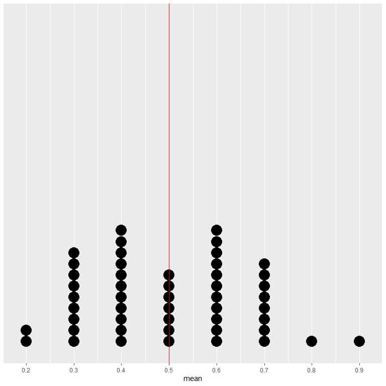
We see a nearly equal number of dots on either side of the vertical line of EV value. Thus, the EV value gives a measure of the data center.

– Example 2

Instead of tossing the coin 10 times, we tossed the coin 50 times and repeat that process 20 times and count the number of heads and the average from every trial.

We will get the following result:

In trial 1, we get 25 heads, so the mean = 25/50 or 0.5.

In trial 2, we get 22 heads, so the mean = 0.44.

The average of heads column = sum of values/ number of trials = 24.65.

The average of mean column = sum of values/ number of trials = 0.493.

If we repeated this process (tossing the coin 50 times) 50 times and count the number of heads and the average from every trial.

We will get the following result:

The average of heads column = sum of values/ number of trials = 24.66.

The average of mean column = sum of values/ number of trials = 0.4932.

We see that:

1. The expected value for the average = probability of success or heads = 0.5 also.

2. The average value converges (get closer) to the EV for the average as we increase the number of trials.

The average value from 20 trials was 0.493, while the average value from 50 trials was 0.4932.

3. The average value of the number of successes gets closer to the EV of the number of successes as we increase the number of trials.

The EV for the number of heads when we toss the coin 50 times = 0.5 X 50 = 25.

The average value from 20 trials was 24.65, while the average value from 50 trials was 24.66.

If we plot the data of 50 trials as a dot plot, we see that EV for the average (0.5) or the EV for the number of heads (25) halves the data distribution.

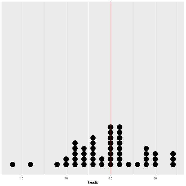
We see a nearly equal number of dots on either side of the vertical line of EV value.

– Example 3

In the following plot, we calculate the average for the different number of tosses starting from 1 toss to 1000 tosses.

In 1 toss, if we get head, so the average = 1/1 = 1.

if we get tail, so the average = 0/1 = 0.

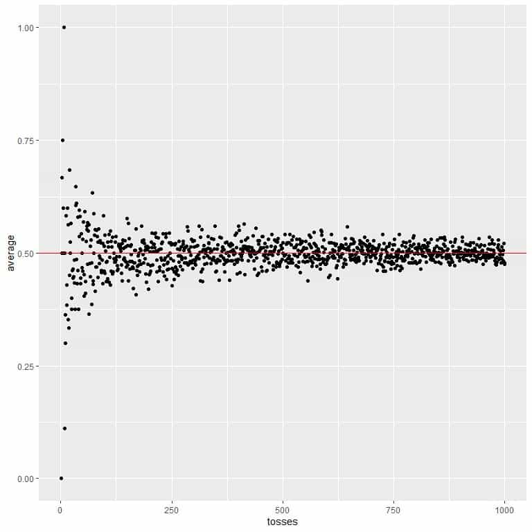
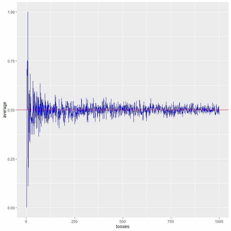
As we increase the number of tosses, the average value, black dots or blue line, becomes closer to the expected value of 0.5, red horizontal line.

Whether we increase the number of trials or the number of tosses within each trial, the average will get closer to the EV for the average.

– Example 4

If we are throwing a fair die, the score we get on the top face is the random variable. There are only six possible outcomes (1,2,3,4,5,or 6). What is the expected value for the average if we rolled this die 10 times?

For a fair die, the probability of 1 = Probability of 2 = Probability of 3 = Probability of 4 = Probability of 5 = Probability of 6 = 1/6.

The expected value for the average = weighted average = 1/6 X 1 + 1/6 X 2 + 1/6 X 3 + 1/6 X 4 + 1/6 X 5 + 1/6 X 6 = 3.5.

We will get the same result if we calculate the average directly = (1+2+3+4+5+6)/6 = 3.5.

We rolled a fair die 10 times, and get the following results:

6 1 5 2 3 6 5 2 3 6.

The average of these values = (6+ 1+ 5+ 2+ 3+ 6+ 5+ 2+ 3+ 6)/10 = 3.9.

If we repeated this process (rolling the die 10 times) 20 times and calculate the average from every trial.

We will get the following result:

The average of trial 1 = 3.3.

The average of trial 2 = 3.2, and so on.

The average of mean column = sum of values/ number of trials = (3.3+ 3.2+ 2.7+ 3.8+ 3.3+ 3.2+ 3.4+ 3.3+ 3.7+ 3.1+ 3.4+ 3.5+ 2.9+ 2.8+ 3.6+ 4.4+ 3.2+ 3.6+ 3.6+ 4.1)/20 = 3.405.

If we repeated this process (rolling the die 10 times) 50 times and calculate the average from every trial.

We will get the following result:

The average of trial 1 = 3.2.

The average of trial 2 = 2.8, and so on.

The average of mean column = sum of values/ number of trials = 3.488.

We see that:

1. The expected value for the average of rolling a die = 3.5.
2. The average value converges (get closer) to the EV for the average as we increase the number of trials.

The average value from 20 trials was 3.405, while the average value from 50 trials was 3.488.

If we plot the data from 50 trials as a dot plot, we see that EV for the average (3.5) halves the data distribution.

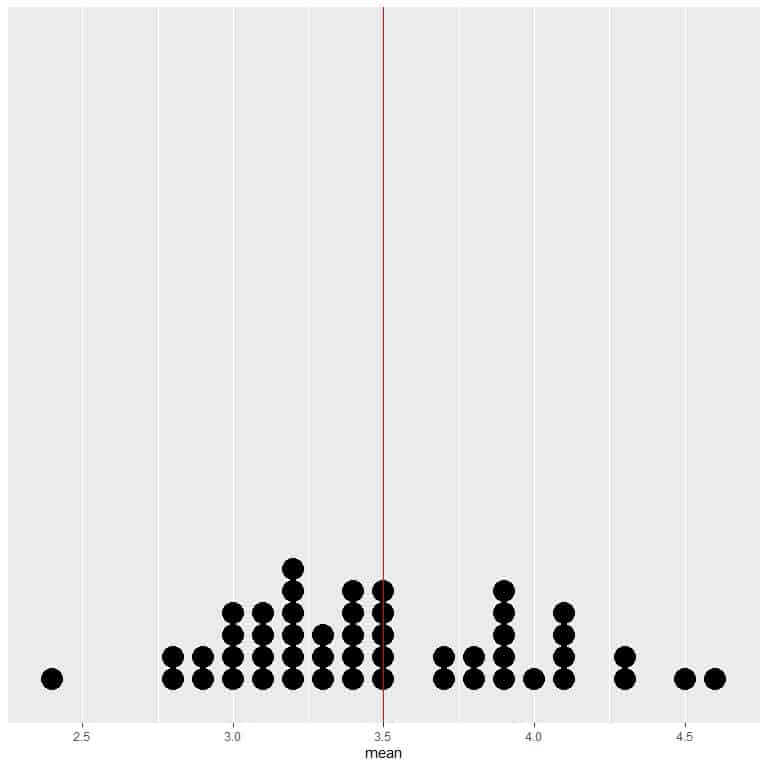
We see a nearly equal number of dots on either side of the vertical line of EV value.

As the number of rollings grows, the average value converges to 3.5, which is the expected value.

We calculate the average for the different number of rolls starting from 1 roll to 1000 rolls in the following plot.

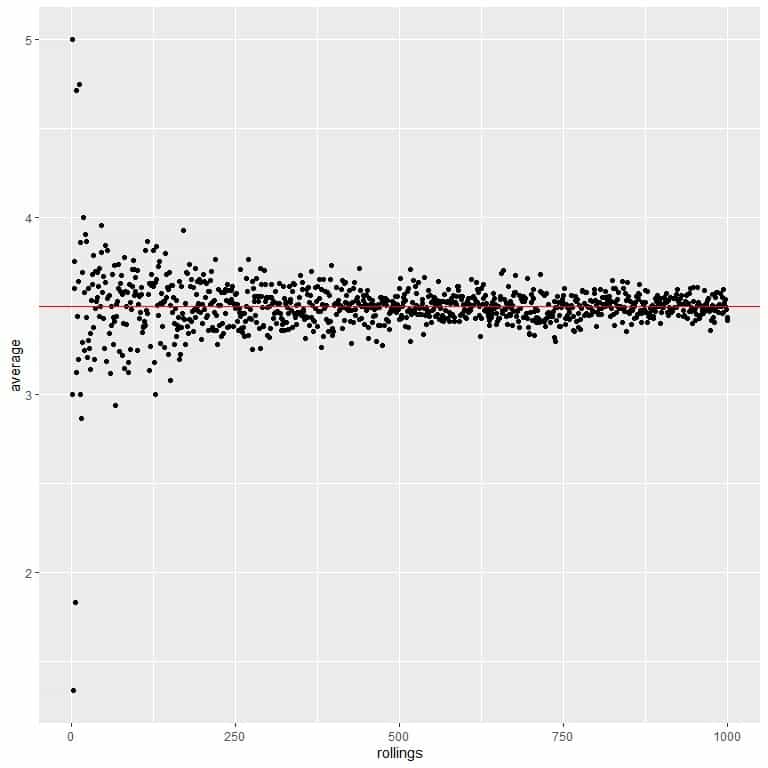
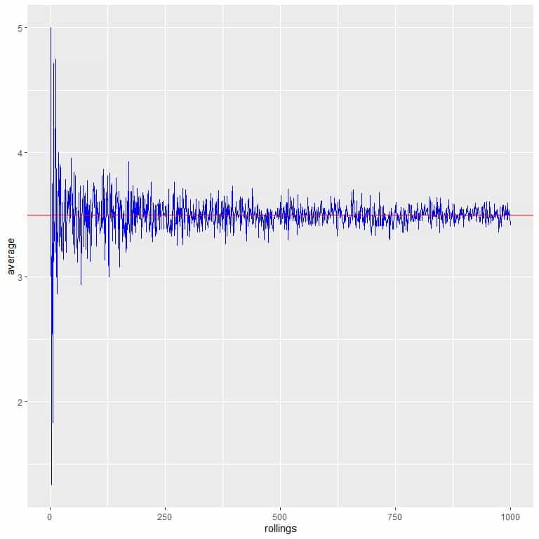
Whether we increase the number of trials or the number of rollings within each trial, the average will get closer to the EV for the average.

The same rules apply to continuous random variables, as we will see in the following example

– Example 3

From the census data, the mean weight of a certain population is 73.44 kg, so the expected value = 73.44.

One group of researchers randomly sample 50 persons from this population and measure their weights, they get the following results:

66.3 70.7 81.0 71.2 59.0 72.0 92.0 83.0 70.5 58.0 83.3 64.0 68.4 68.0 48.5 55.0 55.0 61.0 82.0 62.2 83.0 86.0 78.0 96.0 55.7 58.4 65.0 65.0 72.0 64.0 83.8 71.8 67.0 65.6 74.0 59.0 66.0 81.0 59.0 51.0 70.0 76.5 73.5 74.0 88.0 98.0 63.0 71.8 75.0 55.8.

The mean in this sample = sum of values/sample size = 3518/50 = 70.36.

If we have 20 research groups, each randomly sample 50 persons from this population and calculate the average weight in their respective sample.

We will get the following result:

Research group 1 found a mean = 70.36.

Research group 2 found a mean = 71.844.

Research group 3 found a mean = 74.292.

The average of mean column = 73.047.

If we have 50 research groups, each randomly samples 50 persons from this population and calculates the average weight in their respective sample.

We will get the following result:

The average of mean column = 73.11368.

We see that for a continuous random variable:

1. The expected value for the average = population mean = 73.44.
2. The average value converges (get closer) to the EV as we increase the number of trials or samples.

The average value from 20 trials (20 samples) was 73.047, while the average value from 50 samples was 73.11368.

If we plot the data from 50 samples as a dot plot, we see that EV (73.44) halves the data distribution.

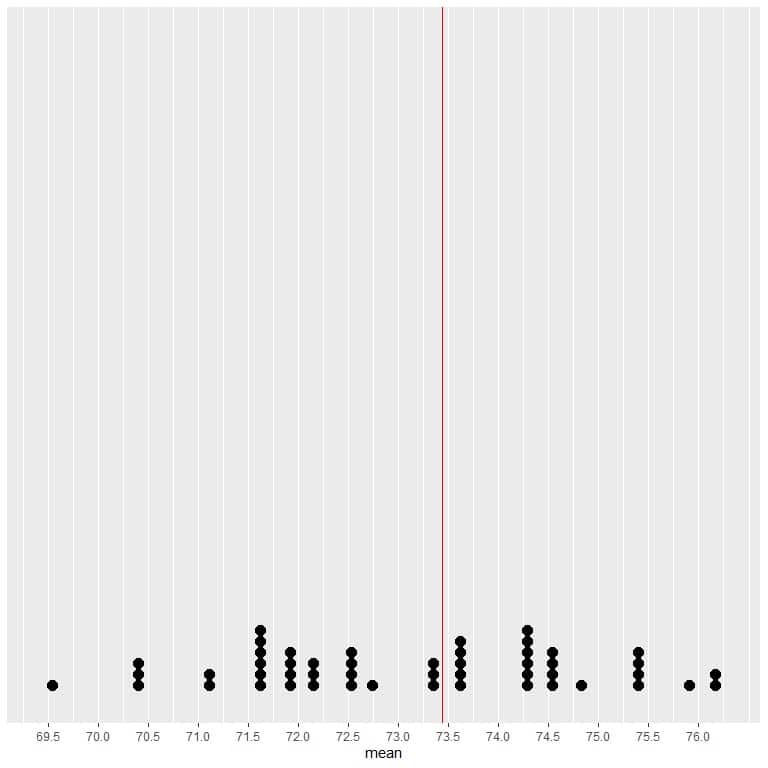
We see a nearly equal number of dots on either side of the vertical line of EV value. Thus, the EV value gives a measure of the data center.

We calculate the average for different sample sizes starting from 1 person to 1000 persons in the following plot.

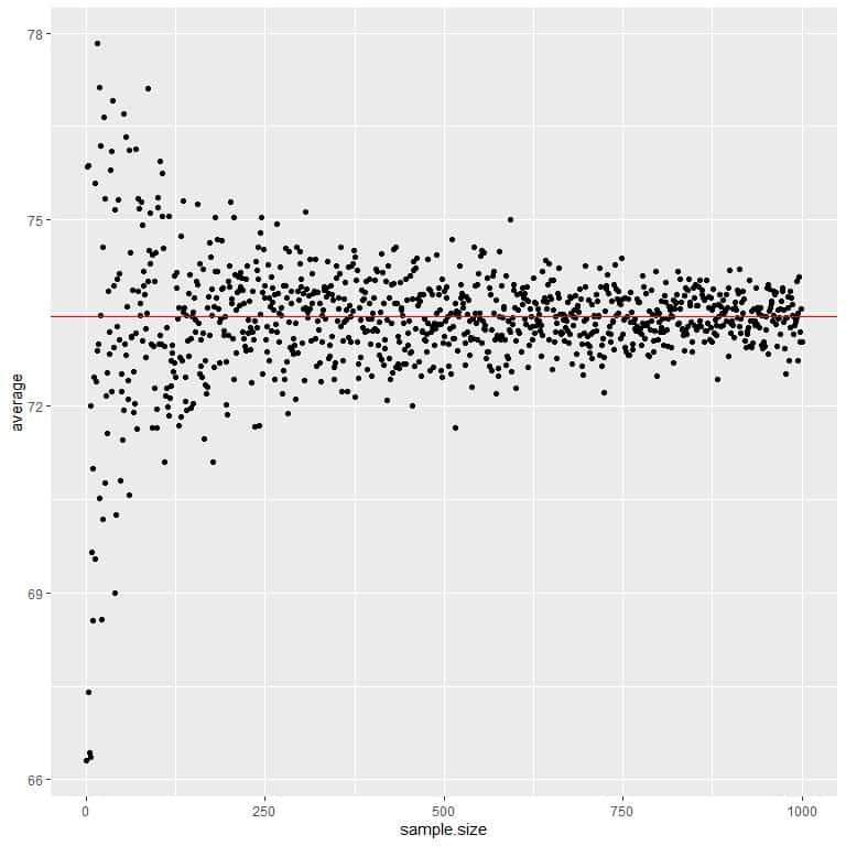
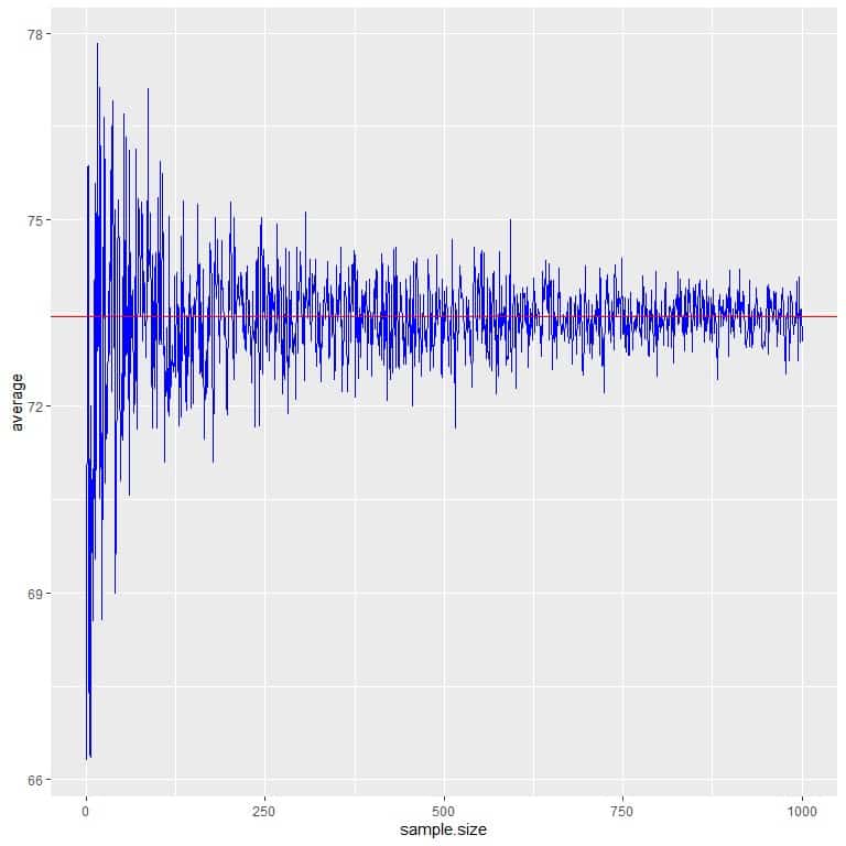
As we increase the sample size, the average value, black dots or blue line, becomes closer to the expected value of 73.44, which we draw as a red horizontal line.

Whether we increase the number of trials (samples) or the number of persons within each sample, the average will get closer to the EV for the average.

How to calculate the expected value?

The expected value of a random variable X, denoted as E[X], is calculated by:

E[X]=∑x_i Xp(x_i)

where:

x_i is an outcome of the random variable.

p(x_i) is the probability of that outcome.

So we multiply each event by its probability then we sum these values to get the expected value.

The expected value formula gives the same result as the formula for calculating the mean.

If we have the population data, we use the population data to calculate each outcome’s probability and the expected value.

If we have sample data, we use the sample mean to estimate the population mean or expected value.

We will go through several examples:

– Example 1

You tossed a coin 50 times and denoted the head as 1 and the tail as 0.

You get the following results:

0 1 0 1 1 0 1 1 1 0 1 0 1 1 0 1 0 0 0 1 1 1 1 1 1 1 1 1 0 0 1 1 1 1 0 0 1 0 0 0 0 0 0 0 0 0 0 0 0 1.

Assuming this is population data, what is the expected value?

Using the expected value formula:

1. We construct a frequency table for each outcome.

2. Add another column for the probability of each outcome.

Probability = frequency/total number of data = frequency/50.

3. Multiply each outcome by its probability and sum to get the expected value.

Expected value = 1 X 0.5 + 0 X 0.5 = 0.5.

Using the mean formula:

The mean = (0+ 1+ 0+ 1+ 1+ 0+ 1+ 1+ 1+ 0+ 1+ 0+ 1+ 1+ 0+ 1+ 0+ 0+ 0+ 1+ 1+ 1+ 1+ 1+ 1+ 1+ 1+ 1+ 0+ 0+ 1+ 1+ 1+ 1+ 0+ 0+ 1+ 0+ 0+ 0+ 0+ 0+ 0+ 0+ 0+ 0+ 0+ 0+ 0+ 1)/50 = 0.5.

So, it is the same result.

When we have a random variable with only two outcomes:

1. The expected value for the average = probability of success = probability of interested outcome.

If we are interested in heads, the expected value = probability of heads = 0.5.

If we are interested in tails, the expected value = probability of tails = 0.5.

2. The expected value for the number of successes = number of trials X probability of success.

If we toss the coin 100 times, the EV of heads = 100 X 0.5 = 50.

If we toss the coin 1000 times, the EV of heads = 1000 X 0.5 = 500.

– Example 2

The following table is the survival data for the 2201 passengers on the ocean liner’s fatal maiden voyage ‘Titanic.’

What is the expected value for the average?

What is the survivors’ expected value if ‘Titanic’ held 100 passengers or 10,000 passengers and ignored all other factors affecting survival (like gender or class)?

1. Add another column for the probability of each outcome.

Probability = frequency / total number of data.

Probability for survival (Survival = Yes) = 711/2201 = 0.32.

Probability for Death (Survival = No) = 1490/2201 = 0.68.

2. We are interested in survival, so we denote “Yes” survival as 1 and “No” survival as 0.

Expected value = 1 X 0.32 + 0 X 0.68 = 0.32.

3. It is a random variable with two outcomes so:

The expected value of the average of survival = probability of interested outcome = probability of survival = 0.32.

The expected value of survived passengers if ‘Titanic’ was holding 100 passengers = number of passengers X probability of survival = 100 X 0.32 = 32.

The expected value of survived passengers for 10,000 passengers = number of passengers X probability of survival = 10000 X 0.32 = 3200.

– Example 3

You are surveying 30 persons for the number of TV hours watched per day.

The TV hours watched per day is a random variable and can take values, 0,1,2,3,4,5,6,7,8,9,10,11,12,13,14,15,16,17,18,19,20,21,22,23, or 24.

Zero means no TV watching at all, and 24 means watching TV at all hours of the day.

You get the following results:

6 9 7 10 11 4 7 10 7 7 11 7 8 8 4 10 6 3 6 11 10 8 8 13 8 8 7 8 6 5.

What is the expected value for the average?

We construct a frequency table for each outcome or number of hours.

If you sum these frequencies, you will get 30 which is the total number of persons surveyed.

For example, there is 1 person who watches TV 3 hours/day.

2 persons watch TV 4 hours/day, and so on.

2. Add another column for the probability of each outcome.

The probability = frequency/total data points = frequency/30.

If you sum these probabilities, you will get 1.

3. Multiply each hour by its probability and sum to get the expected value.

EV = 3 X 0.033 + 4 X 0.067 + 5 X 0.033 + 6 X 0.133 + 7 X 0.2 + 8 X 0.233 + 9 X 0.033 + 10 X 0.133 + 11 X 0.1 + 13 X 0.033 = 7.75.

If we calculate the mean directly, we will get the same result.

The mean = sum of values / the total data number = (6 +9 + 7+ 10+ 11+ 4+ 7+ 10 + 7 + 7+ 11 + 7 + 8+ 8+ 4+ 10+ 6+ 3+ 6+ 11+ 10+ 8+ 8+ 13+ 8+ 8+ 7+ 8 + 6+ 5)/30 = 7.76.

The difference is due to rounding performed when calculating probabilities.

– Example 4

The following are the air pressures (in millibars) at the center of 50 storms.

1013 1013 1013 1013 1012 1012 1011 1006 1004 1002 1000 998 998 998 987 987 984 984 984 984 984 984 981 986 986 986 986 986 986 986 1011 1011 1010 1010 1011 1011 1011 1011 1012 1012 1013 1013 1014 1014 1014 1014 1013 1010 1007 1003.

What is the expected value for the average?

1. We construct a frequency table for each pressure value.

If you sum these frequencies, you will get 50 which is the total number of storms in this data.

2. Add another column for the probability of each pressure.

The probability = frequency/total data points = frequency/50.

If you sum these probabilities, you will get 1.

3. Add another column for the multiplication of each pressure value by its probability.

4. Sum the column of “pressure X probability” to get the expected value.

Sum = Expected value = 1001.58.

If we calculate the mean directly, we will get the same result.

The mean = sum of values / the total data number = (1013+ 1013+ 1013+ 1013+ 1012+ 1012+ 1011+ 1006+ 1004+ 1002+ 1000+ 998+ 998+ 998+ 987+ 987+ 984+ 984+ 984+ 984+ 984+ 984+ 981+ 986+ 986+ 986+ 986+ 986+ 986+ 986+ 1011+ 1011+ 1010+ 1010+ 1011+ 1011+ 1011+ 1011+ 1012+ 1012+ 1013+ 1013+ 1014+ 1014+ 1014+ 1014+ 1013+ 1010+ 1007+ 1003)/50 = 1001.58.

If we plot this data as a dot plot, we see that this number nearly halves the data.

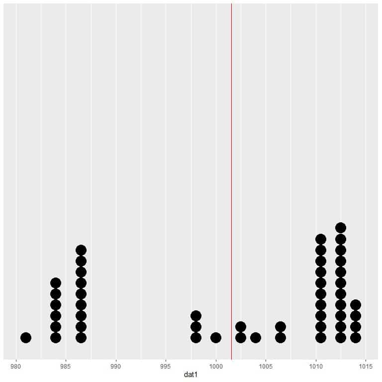
We see a nearly equal number of data points on either side of the vertical line, so the expected value or the mean gives us a measure of the data center.

Properties of expected value

1. For two random variables X and Y:

If y_i=x_i+c, i = 1, 2, . . , n then E[Y]=E[X]+c.

c is a constant value.

Example

x is a random variable with values from 1 to 10.

x = {1, 2, 3, 4, 5, 6, 7, 8, 9, 10}.

E[x] = mean = (1+2+ 3+ 4+ 5+ 6+ 7+ 8+ 9+ 10)/10 = 5.5.

We create another random variable, y, by adding 5 to every element of x.

y = {1+5, 2+5, 3+5, 4+5, 5+5, 6+5, 7+5, 8+5, 9+5, 10+5} = {6, 7, 8, 9, 10, 11, 12, 13, 14, 15}.

E[y] = E[x]+5 = 5.5+5 = 10.5.

If we calculate the mean of y, we will get the same result = (6+ 7+ 8+ 9+ 10+ 11+ 12+ 13+ 14+ 15)/10 = 10.5.

2. For two random variables X and Y:

If y_i=cx_i, i = 1,2, . . . , n then E[Y]=c.E[X].

c is a constant value.

Example

x is a random variable with values from 1 to 10.

x = {1, 2, 3, 4, 5, 6, 7, 8, 9, 10}.

E[x] = mean = (1+2+ 3+ 4+ 5+ 6+ 7+ 8+ 9+ 10)/10 = 5.5.

We create another random variable, y, by multiplying 5 to every element of x.

y = {5, 10, 15, 20, 25, 30, 35, 40, 45, 50}.

E[y] = 5 X E[x] = 5 X 5.5 = 27.5.

If we calculate the mean of y, we will get the same result = (5+10+ 15+ 20+ 25+ 30+ 35+ 40+ 45+ 50)/10 = 27.5.

A common application of this rule, if we know that the expected value for weight from a certain population = 73 kg.

The expected weight in grams = 73 X 1000 = 73000 grams.

3. For two random variables X and Y:

If y_i=c_1 x_i+c_2, i = 1, 2, . . , n then E[Y]=c_1.E[X]+c_2.

c_1 and c_2 are two constants.

Example

x is a random variable with values from 1 to 10.

E[x] = mean = (1+2+ 3+ 4+ 5+ 6+ 7+ 8+ 9+ 10)/10 = 5.5.

We create another random variable, y, by multiplying by 5 and adding 10 to every element of x.

y = {(1 X 5)+10, (2 X 5)+10, (3 X 5)+10, (4 X 5)+10, (5 X 5)+10, (6 X 5)+10, (7 X 5)+10, (8 X 5)+10, (9 X 5)+10, (10 X 5)+10} = {15, 20, 25, 30, 35, 40, 45, 50, 55, 60}.

E[y] = (5 X E[x])+10 = (5 X 5.5)+10 = 37.5.

If we calculate the mean of y, we will get the same result = (15+ 20+ 25+ 30+ 35+ 40+ 45+ 50+ 55+ 60)/10 = 37.5.

4. For random variables Z, X, Y,….:

If z_i=x_i+y_i+…., i = 1, 2, . . , n then E[z]=E[x]+E[y]+……

Example

X is a random variable with values from 1 to 10.

X = {1, 2, 3, 4, 5, 6, 7, 8, 9, 10}.

E[x] = mean = (1+2+ 3+ 4+ 5+ 6+ 7+ 8+ 9+ 10)/10 = 5.5.

Y is another random variable with values from 11 to 20.

Y = {11, 12, 13, 14, 15, 16, 17, 18, 19, 20}.

E[y] = mean = (11+ 12+ 13+ 14+ 15+ 16+ 17+ 18+ 19+ 20)/10 = 15.5.

We create another random variable, Z, by adding every element of X to its respective element from Y.

Z = {1+11,2+12,3+13,4+14,5+15,6+16,7+17,8+18,9+19,10+20} = {12, 14, 16, 18, 20, 22, 24, 26, 28, 30}.

E[Z] = E[X]+E[Y] = 5.5+15.5 = 21.

If we calculate the mean of Z, we will get the same result = (12+ 14+ 16+ 18+ 20+ 22+ 24+ 26+ 28+ 30)/10 = 21.

5. For random variables Z, X, Y,….:

If z_i=c_1.x_i+c_2.y_i+…., i = 1, 2, . . , n. c_1,c_2 are constants:

E[Z]=c_1.E[X]+c_2.E[Y]+……

Example

X is a random variable with values from 1 to 10.

X = {1, 2, 3, 4, 5, 6, 7, 8, 9, 10}.

E[x] = mean = (1+2+ 3+ 4+ 5+ 6+ 7+ 8+ 9+ 10)/10 = 5.5.

Y is another random variable with values from 11 to 20.

Y = {11, 12, 13, 14, 15, 16, 17, 18, 19, 20}.

E[y] = mean = (11+ 12+ 13+ 14+ 15+ 16+ 17+ 18+ 19+ 20)/10 = 15.5.

We create another random variable, Z, by the following formula:

Z = 5 X X + 10 X Y.

Z = {5 X 1+10 X 11,5 X 2+10 X 12, 5 X3+10 X13, 5 X 4+10 X 14, 5 X 5+10 X 15, 5 X 6+10 X 16,5 X 7+10 X 17, 5 X 8+10 X18,5 X 9+ 10 X 19,5 X 10+10 X20} = {115, 130, 145, 160, 175, 190, 205, 220, 235, 250}.

E[Z] = 5.E[X]+10.E[Y] = 5 X5.5+ 10 X15.5 = 182.5.

If we calculate the mean of Z, we will get the same result = (115+ 130+ 145+ 160+ 175+ 190+ 205+ 220+ 235+ 250)/10 = 182.5.

Practice questions

The following is the murder rate (per 100,000 population) for the 50 states of the USA in 1976. What is the expected value for the average?

2. The following is the catholic percentage for each of 47 French-speaking provinces of Switzerland at about 1888. What is the expected value for the average?

3. You randomly sampled 100 individuals from a certain population and asked them for their hypertensive status. You denoted the hypertensive person as 1 and the normotensive individual as 0. You get the following results:

0 1 0 1 1 0 0 1 0 0 1 0 0 0 0 1 0 0 0 1 1 0 0 1 0 1 0 0 0 0 1 1 0 1 0 0 1 0 0 0 0 0 0 0 0 0 0 0 0 1 0 0 1 0 0 0 0 1 1 0 0 0 0 0 1 0 1 1 1 0 1 0 1 0 0 0 0 0 0 0 0 0 0 1 0 0 1 1 1 0 0 0 0 0 0 0 1 0 0 0.

What is the expected value for the average of hypertensive individuals?

What is the expected value for the number of hypertensive individuals if your population size is 10,000?

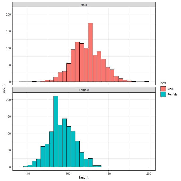
4. The following two histograms are for the heights of females and males from a certain population. Which gender has a higher expected value for the average height?

The following table is the history of hypercholesterolemia for different smoking statuses in a certain population.

What is the expected value for the average disease history for every smoking status?

Answer key

1.We can calculate the mean directly to get the expected value:

The population mean = expected value = sum of numbers/total data = 368.9/50 = 7.378 per 100,000 population.

2. We can calculate the mean directly to get the expected value:

The population mean = expected value = sum of numbers/total data = 1933.76/47 = 41.14%.

3. We can calculate the mean directly to get the expected value:

The expected value for the average = sum of numbers/total data = 29/100 = 0.29.

The expected value for the number of hypertensive individuals if your population size is 10,000 = 0.29 X 10,000 = 2900.

4. We see that males have longer heights (histogram shifted to the right), so males have a higher expected value for the average height.

5. From the table, we extract the proportion of Yes for every smoking status, so:

• For the never smoker, the expected value for the average disease history = 0.32.
• For the current or former < 1-year smoker, the average disease history’s expected value is = 0.25.
• For the former >= 1-year smoker, the expected value for the average disease history = 0.36.

Previous Lesson | Main Page | Next Lesson