JUMP TO TOPIC
Laplace Transform – Definition, Formula, and Applications
 The Laplace transform is an essential operator that transforms complex expressions into simpler ones. Through Laplace transforms, solving linear differential equations can be a breezy process. Numerical methods learned in physics, engineering, and advanced mathematics will always utilize Laplace transforms. In fact, circuit analysis and studying oscillations in physics will not be complete without Laplace transforms.
The Laplace transform allows us to solve constant linear differential equations with ease. We can evaluate the Laplace transform of a function by evaluating its improper integral representation.
In this article, we’ll establish the definition and formula for the Laplace transform. We’ll also show you how to evaluate the Laplace transforms of different functions. Knowing how to work with improper integrals is assumed knowledge in this article, but don’t worry, we’ve added important links throughout the discussion. For now, let’s understand how Laplace transform works!
What Is a Laplace Transform?
The Laplace transform is an important operator when rewriting integrals and solving differential equations. Since the Laplace transforms are mostly used when working with differential equations that represent relationships involving time, we use $t$ and $f(t)$ to represent our functions throughout the discussion.
\begin{aligned}\mathcal{L}\{{f(t)}\} &= F(s) \end{aligned}
We can use $\mathcal{L}$ to represent the Laplace transform operator and $F(s)$ represents the resulting function after working on the Laplace transform of the function, $f(t)$. Here’s how we break down the equation into words:
“The Laplace transform of the function, $f(t)$, is equal to the function, $F(s)$.”
Throughout our discussion, we’ll use the capitalized letter of the function when referring to its Laplace transform.
\begin{aligned}\mathcal{L}\{g(t)\} &= G(s) \\\mathcal{L}\{h(t)\} &= H(s) \\\mathcal{L}\{i(t)\} &= I(s) \end{aligned}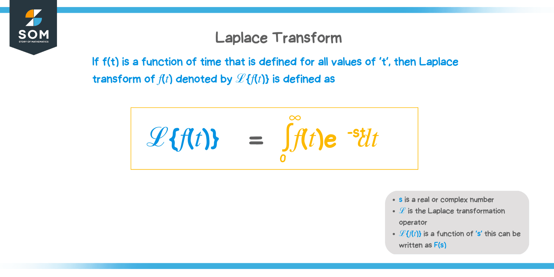
Now, let’s establish the mathematical definition of Laplace transforms and the operator and learn how to set up the Laplace transforms of different functions.
Laplace Transform Definition
Suppose that $f(t)$ is defined for the interval, $t \in [0, \infty)$, the Laplace transform of $f(t)$ can be defined by the equation shown below.
\begin{aligned}\mathcal{L} &= F(s)\\&= \lim_{T \rightarrow \infty} \int_{0}^{T} f(t)e^{-st} \phantom{x}dt\\&= \int_{0}^{\infty} f(t)e^{-st} \phantom{x}dt\end{aligned}
The Laplace transform’s definition shows how the returned function is in terms of $S$. From the equation, we can see that the Laplace transform operator returns an improper integral. As we have learned in the past, the improper integral may or may not converge depending on the resulting integrand. The function can only have a Laplace transform when the resulting improper integral is convergent.
In the next section, we’ll explore common functions’ Laplace transforms and learn how to evaluate these functions using the definition of Laplace transforms.
How To Do Laplace Transforms?
We can use the definition of Laplace transform to find the expressions for the Laplace transforms of common functions.
\begin{aligned}\mathcal{L}\{f(t)\} &= \int_{0}^{\infty} f(t)e^{-st} \phantom{x}dt\end{aligned}
Identify the expression for $f(t)$, then simplify $f(t)e^{-st}$. Integrate the resulting improper integral using appropriate integration techniques you’ve learned in the past. Why don’t we begin by finding the Laplace transform for the function, $f(t) = 1$? We can do thi:
\begin{aligned}\mathcal{L}\{f(t)\} &= F(s) \\&= \int_{0}^{\infty} 1 \cdot e^{-st} \phantom{x}dt\\&= \int_{0}^{\infty} e^{-st} \phantom{x}dt\end{aligned}
When working with improper integrals, we replace $-\infty$ or $\infty$ with a variable, $T$, then evaluate the resulting integral. Evaluate the limit of the expression as $T \rightarrow -\infty$ or $T \rightarrow \infty$.
\begin{aligned}\mathcal{L}\{f(t)\} &= F(s)\\&= \lim_{T\rightarrow \infty}\int_{0}^{T} e^{-st} \phantom{x}dt\\&= \lim_{T\rightarrow \infty} \left(\dfrac{1}{s} -\dfrac{e^{-sT}}{s}\right )\\&= \dfrac{1}{s}\end{aligned}
This Laplace transform exists when $s >0$. We can apply a similar process to establish the Laplace transforms of other common functions. Don’t worry, you can try deriving the rest of the Laplace transform rules in the later section!
Laplace Transform Formula of Common Functions
When working with Laplace transforms of more complex functions, it will be time consuming if we keep deriving the Laplace transform of simple functions each time. This is why having a table of transformations is handy whenever working with problems involving Laplace transforms.
\begin{aligned}\boldsymbol{f(t)}\end{aligned} | \begin{aligned}\boldsymbol{\mathcal{L}\{f(t)\} = F(s)} \end{aligned} |
\begin{aligned} 1\end{aligned} | \begin{aligned} \dfrac{1}{s}, \phantom{x}s > 0\end{aligned} |
\begin{aligned} t^n\end{aligned} | \begin{aligned} \dfrac{n!}{s^{n +1}},\phantom{x}s > 0\end{aligned} |
\begin{aligned} e^{kt}\end{aligned} | \begin{aligned} \dfrac{1}{s – k}, \phantom{x}s > k\end{aligned} |
\begin{aligned} \sin (ct)\end{aligned} | \begin{aligned} \dfrac{c}{s^2 + c^2},\phantom{x}s > 0\end{aligned} |
\begin{aligned} \cos (ct)\end{aligned} | \begin{aligned} \dfrac{s}{s^2 + c^2}, \phantom{x}s > 0\end{aligned} |
\begin{aligned} \sinh (ct)\end{aligned} | \begin{aligned} \dfrac{c}{s^2 – c^2},\phantom{x}s >\pm c\end{aligned} |
\begin{aligned} \cosh (ct)\end{aligned} | \begin{aligned} \dfrac{s}{s^2 – c^2}, \phantom{x}s > \pm c\end{aligned} |
\begin{aligned} y^{\prime }\end{aligned} | \begin{aligned} sF(s) – f(0), \phantom{x}s > 0\end{aligned} |
\begin{aligned} y^{\prime\prime}\end{aligned} | \begin{aligned} s^2F(s)– sf(0) – f^{\prime}(0), \phantom{x}s > 0\end{aligned} |
\begin{aligned} y^{(n) }\end{aligned} | \begin{aligned} s^nF(s) – s^{n -1}f(0)- s^{n -2}f^{\prime}(0)… -sf^{(n -2)}(0)– f^{(n -1) }(0), \phantom{x}s > 0\end{aligned} |
These are just some of the many functions with Laplace transforms. You can even list more on your own and try to derive their Laplace transform based on the definition you’ve just learned of Laplace transforms. We’ve prepared more examples for you to work on as well!
Example 1
What is the Laplace transform of the function, $f(t) = t$? Confirm that this is true given that the Laplace transform of $f(t) = t^n$ is equal to $F(s) =\dfrac{n!}{s^{n +1}}$.
Solution
Use the definition for Laplace transforms given the expression for $f(t) = t$.
\begin{aligned}f(t) &= t\\\mathcal{L}\{t\} &= \int_{0}^{\infty} te^{-st} \phantom{x}dt\\&= \lim_{T\rightarrow \infty} \int_{0}^{T} te^{-st} \phantom{x}dt\end{aligned}
Apply $u$-substitution and integration by parts to integrate our expression. Evaluate the integral using the lower and upper limits: $t = 0$ and $t = T$.
\begin{aligned}\int te^{-st} \phantom{x}dt &= \dfrac{1}{s^2} \int ue^u \phantom{x}du \phantom{x}(u = -st)\\&= \dfrac{1}{s^2}\left(e^uu-\int \:e^udu\right)\\&= \dfrac{1}{s^2}\left(e^uu-e^u\right)\\&= \dfrac{1}{s^2}\left(-se^{-st}t-e^{-st}\right)\\\\\int_{0}^{T} te^{-st} \phantom{x}dt &= \dfrac{1}{s^2}\left(-se^{-st}t-e^{-st}\right)|_{0}^{T}\\&= \dfrac{1}{s^2}(-Tse^{-Ts}-e^{-Ts}+1)\end{aligned}
Evaluate our expression’s limit and see what happens when $T \rightarrow \infty$.
\begin{aligned}\mathcal{L}\{t\}&= \lim _{T\rightarrow \infty}\left[ \dfrac{1}{s^2}(-Tse^{-Ts}-e^{-Ts} +1)\right ]\\&=\dfrac{1}{s^2} \lim_{T\rightarrow \infty}\left[ (-Tse^{-Ts}-e^{-Ts} +1)\right ]\\&= \dfrac{1}{s^2}(0 + 0 + 1)\\&= \dfrac{1}{s^2}, \phantom{x}s >0\end{aligned}
This means that the Laplace transform of $f(t) = t$ is equal to $F(s) = \dfrac{1}{s^2}$. Let’s now use the Laplace transform formula for $ f(t) = t^n$, where $n = 1$:
\begin{aligned}F(s)&= \mathcal{L}\{t^1\}\\&= \dfrac{1!}{s^{1 +1}}\\&= \dfrac{1}{s^2}\end{aligned}
The Laplace transform formula still holds true and this example shows you how important it is to know the table of Laplace transforms if you want to work with more complex problems later.
Example 2
Find the Laplace transforms of the following functions:
a. $f(t) = 3e^{-4t} + e^{2t} + 6t^4 -6$
b. $g(t) = 6\cos (2t) + 3\sin (6t) – 12 $
Solution
There are instances when the function we’re working with contains multiple terms, so let’s establish a rule when evaluating their Laplace transforms. When given, $f(t)$ and $g(t)$, we have the following:
\begin{aligned}\mathcal{L}\{af(t) + bg(t)\} &= aF(s) + bG(s)\end{aligned}
This means that the constant factors won’t be a problem for us, nor will the operations in between. For the first function, $f(t) = 3e^{-4t} + e^{2t} + 6t^4 -6$, we can work on the Laplace transforms of each term, then just combine the resulting expressions.
\begin{aligned}\boldsymbol{3e^{-4t}}\end{aligned} | \begin{aligned}\boldsymbol{e^{2t}}\end{aligned} | \begin{aligned}\boldsymbol{6t^4}\end{aligned} | \begin{aligned}\boldsymbol{-6}\end{aligned} |
\begin{aligned}\mathcal{L}\{3e^{-4t}\} &= 3\mathcal{L}\{e^{-4t}\}\\&=3 \cdot \dfrac{1}{s – (-4)}\\&= \dfrac{3}{s + 4} \end{aligned} | \begin{aligned} \mathcal{L}\{e^{2t}\} &= \dfrac{1}{s – 2} \end{aligned} | \begin{aligned}\mathcal{L}\{6t^4\} &= 6\mathcal{L}\{t^4\}\\&= 6 \cdot \dfrac{4!}{s^{4 + 1}}\\&= \dfrac{144}{s^5} \end{aligned} | \begin{aligned}\mathcal{L}\{6\} &= 6\mathcal{L}\{1\}\\&= 6 \cdot \dfrac{1}{s}\\&= \dfrac{6}{s} \end{aligned} |
\begin{aligned} F(s) &= \mathcal{L}\{3e^{-4t}\} + \mathcal{L}\{e^{2t}\} + \mathcal{L}\{6t^4\} – \mathcal{L}\{6\}\\&= \dfrac{3}{s + 4} +\dfrac{1}{s – 2} +\dfrac{144}{s^5} -\dfrac{6}{s} \end{aligned} | |||
This means that the Laplace transform is equal to $F(s) = \dfrac{3}{s + 4} +\dfrac{1}{s – 2} +\dfrac{144}{s^5} -\dfrac{6}{s}$.
We can apply a similar process for the next two items, so let’s go ahead and work on the Laplace transform of $g(t)$.
\begin{aligned}\boldsymbol{6\cos (2t)}\end{aligned} | \begin{aligned}\boldsymbol{3\sin (6t) } \end{aligned} | \begin{aligned}\boldsymbol{12}\end{aligned} |
\begin{aligned}\mathcal{L}\{6\cos (2t)\} &= 6\mathcal{L}\{\cos (2t)\}\\&=6 \cdot \dfrac{s}{s^2 + (2)^2}\\&= \dfrac{6s}{s^2 + 4} \end{aligned} | \begin{aligned}\mathcal{L}\{3\sin(6t)\} &= 3\mathcal{L}\{\sin(6t)\}\\&=3 \cdot \dfrac{6}{s^2 + (6)^2}\\&= \dfrac{18}{s^2 + 36} \end{aligned} | \begin{aligned}\mathcal{L}\{12\} &= 12\mathcal{L}\{1\}\\&= 12 \cdot \dfrac{1}{s}\\&= \dfrac{12}{s} \end{aligned} |
\begin{aligned} G(s) &= \mathcal{L}\{6\cos (2t)\} +\mathcal{L}\{3\sin(6t)\} – \mathcal{L}\{12\}\\&= \dfrac{6s}{s^2 + 4} + \dfrac{18}{s^2 + 36} +\dfrac{12}{s} \end{aligned} | ||
Hence, the Laplace transform is equal to $G(s) = \dfrac{6s}{s^2 + 4} + \dfrac{18}{s^2 + 36} +\dfrac{12}{s} $.
Practice Questions
1. Show that the Laplace transform of $f(t) = e^{kt}$ is equal to $F(s) = \dfrac{1}{ s – k}$, where $s > k$.
2. Find the Laplace transforms of the following functions:
a. $f(t) = 2e^{-4t} – e^{3t} +4t^6 – 8$
b. $g(t) = 2\sin (3t) – 4\cos (8t) + 6 $
c. $h(t) = e^{3t} – \cos (4t) – e^{3t}\sin (6t)$
2. Show that the Laplace transform of $f(t) = \cos ct$ is equal to $F(s) = \dfrac{s}{ s^2 + c^2}$, where $s > 0$.
Answer Key
1.
$ \begin{aligned}\mathcal{L}\{e^{kt}\} &= \int_{0}^{\infty} e^{-(s – k)t} \phantom{x}dt\\&= \lim_{T \rightarrow \infty}\int_{0}^{T} e^{-(s – k)t} \phantom{x}dt\\&= \left\{\begin{matrix} T, \phantom{xxxxxxxx}s= k\\ \dfrac{1 – e^{-(s -k)T}}{s – k}, s \neq k\end{matrix}\right. \end{aligned}$
When $s > k$, we have $F(s) = \dfrac{1}{s – k}$.
2.
a. $F(s) = \dfrac{2}{s+4}- \dfrac{1}{s-3} +\dfrac{2880}{s^7}- \dfrac{8}{s}$
b. $G(s) = \dfrac{6}{s^2+9}- \dfrac{4s}{s^2+ 64} + \dfrac{6}{s}$
c. $H(s) = \dfrac{1}{s -3} – \dfrac{s}{s^2 + 16}- \dfrac{6}{\left(s – 3\right)^2 + 36}$
3.
$\begin{aligned}\mathcal{L}\{\cos (ct)\} &= \int_{0}^{\infty} e^{-st} \cos ct \phantom{x}dt\\&= \lim_{T \rightarrow \infty} \int_{0}^{T} e^{-st} \cos ct \phantom{x}dt\phantom{x}dt\\&= \lim_{T \rightarrow \infty} \left[\dfrac{e^{-st}(-s\cos ct + c \sin ct)}{(-s)^2 + c^2} \right ]_{0}^{L}\\&= \dfrac{s}{s^2 + c^2}\end{aligned}$