Limits Calculus – Definition, Properties, and Graphs

Limits are the foundation of calculus – differential and integral calculus. Predicting and approximating the value of a certain set of quantities and even functions is an important goal of calculus. This means that learning about limits will pave the way for a stronger foundation and better understanding of calculus.

Limits reflect the value that a given function approaches when it’s near a certain point.

Limits are most helpful when we want to find a function’s value as it approaches a restricted value. Isn’t it amazing how we can approximate a value as $x$ approaches infinity through different math concepts?

Needless to say, if you want to appreciate higher math classes, mastering limits and their foundations will be essential, and that’s what we’re going to explore in this article.

In this article, we’ll explore the fundamental definition of limits, refresh what we’ve learned about evaluating limits, recall the different limit laws, and visualize limits on an $xy$-plane.

What is a limit?                

The definition of limit can be summarized by the equation:

\begin{aligned}\lim_{x \rightarrow a} f(x) &= L \end{aligned}

Let’s say we have $f(x)$ and it’s close to a unique number, $L$, as $x$ approaches $a$ on both sides, we can define the limit of $f(x)$ as $x$ approaches $a$ is represented by $L$.

We can better understand its definition by observing a given function’s graph as the input value approaches or is near a certain value.

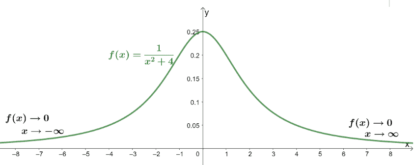
The graph of $f(x) = \dfrac{1}{x^2 + 4}$ is as shown above and we can see that when $x$ approaches a significantly large value, $f(x)$ approaches the $x$-axis. This means that as $x \rightarrow \infty$, $f(x) \rightarrow 0$.

We can actually observe a similar behavior when $x$ approaches a significantly small value – the function approaches zero. 

We can say that the limit of $f(x)$ as $x$ approaches infinity is equal to zero. This confirms the definition of limits.

Let’s apply this definition to understand why $\lim_{x \rightarrow 0} \dfrac{\sin x}{x} = 1$ given the graph of $y = \dfrac{\sin x}{x}$ as shown below.

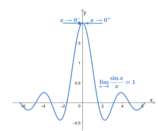
Seeing that the function is near $1$ when $x$ approaches $0$ from either side, we can see that the function’s limit as $x$ approaches $0$ is equal to $1$, indeed. This definition of a limit is informal since we’re only considering limits as $x$ is  “approaching” or is “closer to” a specific value.

In short, we are not definite with our idea of proximity. This is why we’ll also explore the more authoritative and precise definition of a limit in Calculus. This can help us understand the technicalities of different properties that involve limits.

A precise definition of a limit

We’ll lay out the formal definition of a limit in this section and break down each component.

If $L$ represents the limit of $f(x)$ as $x$ approaches $a$, if it satisfies the following conditions:

1. i) Although it’s not necessary for $f(x)$ to be defined at $x = a$, $f(x)$ must still be defined for some interval that contains $x = a$.
2. ii) For every $\epsilon > 0$, we can find a $\delta$ such that $\delta$ is also greater than $0$, so that for all the values of $x$ within the domain of $f(x)$, we have the following:

\begin{aligned}|x -a|< \delta\\\Rightarrow |f(x) – L| < \epsilon \end{aligned}

Let’s break down the conditions to better understand the formal definition of limits.

• The absolute value expression, $|x -a|$, represents the distance between $x$ and $a$, so $|x -a| <  \delta$ means that we want the distance to between the two to be less than $\delta$.
• The value, $\epsilon$, represents the proximity of $\epsilon$ with $f(x)$ so we can approximate the value of $L$.
• Meanwhile, $\delta$ represents the distance or how close you want $x$ and $a$ to be.

This means that we can determine and confirm the limit of a given function by assuming that we have $\epsilon > 0$, and so, we need to find $\delta$ so that the inequalities hold true.

For example, if we want to prove that $\lim_{x \rightarrow 6} -3x + 2 = -16$ using the formal definition of a limit, we have the following components:

\begin{aligned}f(x) &= -3x + 2\\a&= 6\\L &= -16\end{aligned}

We want to make sure that $|f(x) – L| < \epsilon$, where $\epsilon$ is the accepted minimum difference we have set.

\begin{aligned}|f(x) –  L| &= |(-3x + 2) – (-16)|\\&= |-3x + 2 + 16|\\&= |-3x + 18|\\&= |-3| \cdot |x -6|\\&= 3|x – 6|\end{aligned}

Since we have $|f(x) – L| < \epsilon$ and consequently, $3|x – 6| < \epsilon$.

\begin{aligned}3|x – 6| < \epsilon\\|x – 6| < \dfrac{1}{3}\epsilon\end{aligned}

For us to confirm that $\lim_{x \rightarrow 6} f(x) = -16$, we can use $\delta = \dfrac{1}{3} \epsilon$. Hence, we have the inequality shown below.

\begin{aligned}|x – 6| < \dfrac{1}{3}\epsilon\\|x- 6|<\delta\phantom{x}\end{aligned}

Both $\epsilon$ and $\delta$ will always be greater than zero. Hence, we’ve satisfied the condition that when $|x – 6| < \dfrac{1}{3} \epsilon$ and consequently, $|x – 6| < \delta$, we can guarantee that $|(-3x + 2) – (-16)|< \epsilon$.  This confirms the fact that $\lim_{x\rightarrow 6} -3x + 2$ is indeed $-16$.

Now that we’ve explored the informal and formal definitions of limits let’s review the different methods we can apply to evaluate the limits of different functions.

How to do limits?                

There are different ways for us to evaluate limits – and our chosen method will depend on what we’re given. We can evaluate the limits of a given function by its table of values, graphs, and expressions.

This section will help you review your past knowledge of limits from your precalculus classes and learn new techniques to evaluate complicated expressions and functions’ limits.

Observing the limit of a function using its graph or table of values

When given the function’s graph or the table of values to find the limit of a graph, it’s helpful to use the fact that we’re looking for the value of $f(x)$ as $x$ approaches $a$ from both sides.

We’ve shown how we can determine the limit of functions using their graphs, so let’s try finding $\lim_{x \rightarrow 4} -\dfrac{2}{x – 2}$ using the table of values for $y  = -\dfrac{2}{x- 2}$. Make sure to use values of $x$ that are significantly close to $x = 4$ as shown below.

We can see that as $x$ approaches $4$ from the left (these are the values that are less than $4$) , we can see that $f(x)$ is approaches $-1$. The same behavior happens $x$ approaches $4$ from the right. This means that $\lim_{x \rightarrow 4} -\dfrac{2}{x – 2} = -1$.

This approach is only convenient when the graph or the table of values is given. However, there are instances that it’ll be tedious for us to graph or construct a function’s table of values. This is why it’s important we can evaluate limits using different algebraic properties.

Applying the limit laws and evaluating limits

It’s important to master the limit laws we’ve established in the past to understand how we can evaluate limits using different algebraic manipulations we’ve learned in our precalculus classes.

Here’s a summary of the different limit laws we can apply when evaluating limits and checking the corresponding examples to ensure you can apply these laws whenever necessary.

These limit laws, alone, are not enough to evaluate the limits of complex expressions, so we’ve come up with different techniques we can apply to evaluate limits. These techniques are algebraic properties we’ve actually learned in the past, so it’s also a great avenue for us to review our previous knowledge.

As a refresher, let’s discuss the most commonly applied techniques when evaluating limits:

• Direct substitution: Whenever possible, substitute $a$ into $f(x)$ to find $\lim_{x \rightarrow a} f(x)$.

\begin{aligned}\lim_{x \rightarrow a} f(x) &= f(a)\\\\\lim_{x \rightarrow \color{green}3} x^2 – 1 &= ({\color{green}3})^2 -1\\&= 9 -1\\&= 8 \end{aligned}

• Factoring the function: When direct substitution leads to $\dfrac{0}{0}$ or $\dfrac{k}{0}$, we can try factoring out the expression to see if we can cancel out common factors.

\begin{aligned}\lim_{x \rightarrow 1} \dfrac{x^2 -1}{x^2 – 3x + 2} &=\lim_{x \rightarrow 1}  \dfrac{(x -1)(x + 1)}{(x -1)(x – 2)}\\&= \lim_{x \rightarrow 1}  \dfrac{\cancel{(x – 1)}(x +1)}{\cancel{(x – 1)}(x -2)}\\&= \lim_{x \rightarrow \color{green} 1} \dfrac{x + 1}{x -2}\\&= \dfrac{{\color{green}1} + 1}{{\color{green}1} -2}\\&= -2\end{aligned}

• Reversing a rationalized radical expression: When we have a radical expression, we can multiply the numerator and denominator by the numerator’s conjugate.

\begin{aligned} \lim_{x \rightarrow 4}\dfrac{\sqrt{x} – 2}{x – 4} &= \lim_{x \rightarrow 4}\dfrac{\sqrt{x} – 2}{x – 4} \cdot \dfrac{\color{green} \sqrt{x} + 2}{\color{green} \sqrt{x} + 2}\\&= \lim_{x \rightarrow 4} \dfrac{(\sqrt{x} – 2)({\color{green} \sqrt{x} + 2})}{(x – 4)({\color{green} \sqrt{x} + 2})}\\&= \lim_{x \rightarrow 4} \dfrac{(\sqrt{x})^2 – (2)^2}{(x – 4)(\sqrt{x} +2)},\phantom{xxx} (a -b)(a +b) = a^2 – b^2\\ &=\lim_{x \rightarrow 4} \dfrac{\cancel{x – 4}}{\cancel{(x -4)}(\sqrt{x} +2)}\\&= \lim_{x \rightarrow 4} \dfrac{1}{\sqrt{x} +2}\\&= \dfrac{1}{\sqrt{\color{green}4}+ 2}\\&= \dfrac{1}{4}\end{aligned}

• Be creative and manipulate algebraic expressions: There are instances where we need to be creative and apply different algebraic properties to evaluate a function’s limits.

Evaluating one-sided limits and continuous functions

There are instances where $f(x)$ approaches different values as $x$ approaches $a$ from the left and from the right.  We call these limits as one-sided limits – $\lim_{x \rightarrow a^{-}} f(x)$ and $\lim_{x \rightarrow a^{+}} f(x)$.

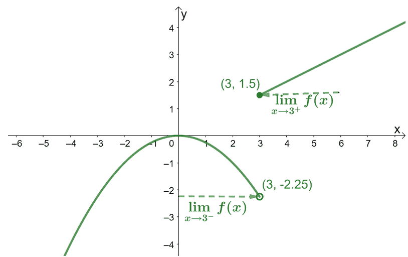
Here’s an example of a function, $f(x)$, where the limits may vary as $x$ approaches from the left and when $x$ approaches from the right.

• One-sided limit from the left: to find $\lim_{x \rightarrow a^{-} f(x)}$, we simply observe the value that $f(x)$ approaches when $x$ approaches $a$ from the left. This means that $\lim_{x\rightarrow 3^{-}} f(x) = -2.25$.
• One-sided limit from the right: similarly,to find $\lim_{x \rightarrow a^{+}}$, we find the value that $f(x)$ approaches when $x$ approaches $a$ from the right. Hence, $\lim_{x\rightarrow 3^{+}} f(x) = 1.5$.

Knowing the one-sided limits of a function can help us determine whether it is continuous or not. To learn more about continuous functions, check out this link here. What’s important is to remember the fact that when $\lim_{x \rightarrow a^{-} f(x)} = \lim_{x \rightarrow a^{+} f(x)}$, the function is continuous.

Using the Squeeze theorem to evaluate complex functions

There are instances where evaluating limits using algebraic manipulation can be challenging – especially when these functions are oscillating. When this happens, we can use the Squeeze theorem to evaluate these limits. As a refresher, we can apply these steps below:

• Begin by confirming three functions such that $g(x) \leq f(x) \leq h(x)$, the limits of $g(x)$ and $h(x)$ as $x \rightarrow a$ are easy to evaluate, and these limits are equal.
• Start with an inequality that’s easy to manipulate, then modify it so that we end with $f(x)$ – the actual function that we’re evaluating.
• Evaluate the limits of the inequalities’ two ends and use the limits to find $\lim_{x\rightarrow a} f(x)$.

We can use the Squeeze theorem to determine limits of complex trigonometric functions such as $\lim_{x\rightarrow 0} \dfrac{\sin x}{x}$ and $\lim_{x\rightarrow 0} \dfrac{ 1- \cos x}{x}$. Why don’t we go ahead and summarize all trigonometric functions’ limits?

How to graph limits?                

Now that we’ve thoroughly explored the concepts of limits and the different methods we can evaluate a function’s limits, we can reverse the process and learn how we can graph limits depending on the limits’ nature.

We’ve learned that discontinuities can either be a hole, asymptotes, or jump discontinuities in our discussion of continuous functions.

• Jump discontinuities occur when the one-sided limits are not the same such as piece-wise functions.
• Holes or removable discontinuities occur when the limit still exists and can be evaluated by canceling common factors shared by the numerator and the denominator.
• Asymptotes or infinite discontinuity happens when the resulting limit of a function as $x$ approaches $a$ is equal to $\pm \infty$. When this happens, we have a vertical asymptote at $x =a$.

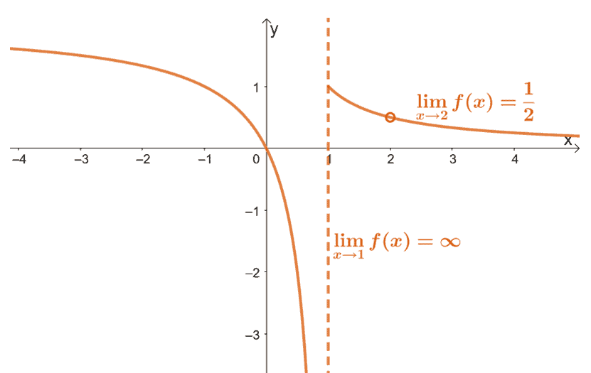
We can use these to graph the limits and represent them on an $xy$-coordinate system. For example, if we have a piecewise function, $f(x)=\left\{\begin{matrix}2 + \dfrac{2}{x -1},&x\leq1\\ \dfrac{x -2}{x^2 – 2x},&x >1\end{matrix}\right.$. The limits of $f(x)$ as $x$ approaches $1$ and $2$ as shown below:

Knowing the nature of the discontinuity can help us identify how it will represent its limit’s value on the graph.

We can apply a similar approach to graph different limits – make sure to review our past knowledge on limits and continuous functions. To further solidify our knowledge of limits, let’s go ahead and try out these sample problems!

Example 1

The graph of $\dfrac{-4x^2 +x}{x}$ is shown below.

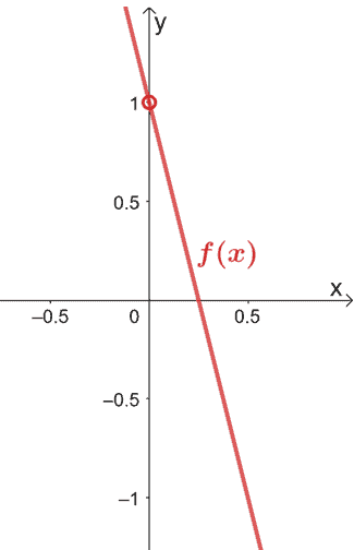
Determine the limit (if it exists) of the function as $x$ approaches the following:
a. $\lim_{x\rightarrow 0} f(x)$
b. $\lim_{x\rightarrow 0.25} f(x)$
c. $\lim_{x\rightarrow 0.5} f(x)$

Solution

When given the graph of the function, we can observe where the function is approaching as $x$ approaches a given value.

We can see that there’s a hole at $(0, 1)$, and we can see that as $x$ approaches $0$ from both sides, $f(x)$ will be approaching $1$. This means that $\lim_{x\rightarrow 0} f(x) = 1$.

We can apply a similar approach for the next two items:

• We can see that as $x$ approaches $0.25$ from both sides, the function approaches $0$. This means that $\lim_{x\rightarrow 0.25} f(x) = 0$.
• Similarly, as $x$ approaches $0.5$, we can see that $f(x)$ approaches $-1$, so $\lim_{x\rightarrow 0.5} f(x) = -1$.

Example 2

Create a table of values (feel free to use a calculator) for the following functions, then approximate the limits of the functions to three decimal places.

a. $\lim_{x\rightarrow 0} \dfrac{1- e^{-2x}}{x}$
b. $\lim_{x\rightarrow 0} (1 – x)^{\frac{1}{x}}$
c. $\lim_{x\rightarrow 16} \dfrac{4 – \sqrt{x}}{x – 16}$

Solution

Since we want to find the limit of $\dfrac{1- e^{-2x}}{x}$ as $x$ approaches $0$, so we can create a table of values that shows $x$ that are significantly close to $0$.

We can see that as $x$ approaches $0$ from the left, $f(x)$ approaches $2.000$. Similarly, as $x$ approaches $0$ from the right, the function also approaches $2.000$. This means that $\lim_{x\rightarrow 0} \dfrac{1- e^{-2x}}{x} = 2$.

We’ll apply a similar process to approximate the limit of $(1 – x)^{\frac{1}{x}}$ as $x$ approaches $0$.

From this, we can see that $f(x)$ approaches $0.368$ as $x$ approaches $0$ from both sides, so $\lim_{x\rightarrow 0} (1 – x)^{\frac{1}{x}} \approx 0.368$.

Let’s work on the third function, $\dfrac{4 – \sqrt{x}}{x – 16}$, and find the values of $x$ that are significantly close to $16$.

This table of values shows that when $x$ is close to $16$, we can see that $f(x)$ is approaching $-0.125$, so $\lim_{x\rightarrow 0} (1 – x)^{\frac{1}{x}} \approx -0.125$.

Example 3

Evaluate the limit (if it exists) of the following functions.

a. $\lim_{x\rightarrow 2} -\dfrac{x}{4}$
b. $\lim_{x\rightarrow 5} \dfrac{x -5}{x^2 – 25}$
c. $\lim_{x\rightarrow 3} \dfrac{x^{4} – 81}{x – 3}$
d. $\lim_{x\rightarrow 0} \dfrac{\dfrac{1}{x + 2} – \dfrac{1}{2}}{x}$

Solution

When given the function, we can always begin by direct substitution if we think that the denominator won’t be equal to zero like the first item, $\lim_{x\rightarrow 2} -\dfrac{x}{4}$. Hence, we have the following:

\begin{aligned}\lim_{x\rightarrow 2} -\dfrac{x}{4} &= – \dfrac{\color{green} 2}{4}\\&= -\dfrac{1}{2}\end{aligned}

Direct substitution won’t apply for the second item since $x^2 – 25 = 0$ when $x = 5$. What we can do is factor the denominator first using the algebraic property, $a^2 – b^2 = (a- b)(a + b)$.

\begin{aligned}\lim_{x\rightarrow 5} \dfrac{x -5}{x^2 – 25} &=\lim_{x\rightarrow 5} \dfrac{x -5}{(x – 5)(x + 5)}\\ &=\lim_{x\rightarrow 5} \dfrac{\cancel{x -5}}{\cancel{(x – 5)}(x + 5)} \end{aligned}

We can then cancel out the common factor shared by the numerator and denominator and see if we can apply direct substitution after.

\begin{aligned}\lim_{x\rightarrow 5} \dfrac{1}{(x + 5)} &= \dfrac{1}{{\color{green}5} + 5}\\&= \dfrac{1}{10} \end{aligned}

We can a similar process to find $\lim_{x\rightarrow 3} \dfrac{x^{4} – 81}{x – 3}$

by factoring the $x^4 – 81$ completely.

\begin{aligned}\lim_{x\rightarrow 3} \dfrac{x^{4} – 81}{x – 3} &= \lim_{x\rightarrow 3} \dfrac{(x^2 -9)(x^2 + 9)}{x – 3}\\&= \lim_{x\rightarrow 3} \dfrac{(x -3)(x + 3)(x^2 + 9)}{x – 3}\\ &= \lim_{x\rightarrow 3} \dfrac{\cancel{(x -3)}(x + 3)(x^2 + 9)}{\cancel{x – 3}}\\&= \lim_{x\rightarrow 3}(x + 3)(x^2 + 9)\end{aligned}

We can now substitution $x = 3$ into the simplified expression so that we can find the limit of the function.

\begin{aligned}\lim_{x\rightarrow 3}(x + 3)(x^2 + 9) &= ({\color{green} 3} + 3)[({\color{green} 3})^2 +9]\\&= 6(18)\\&= 108\end{aligned}

Finding $\lim_{x\rightarrow 0} \dfrac{\dfrac{1}{x + 2} – \dfrac{1}{2}}{x}$ is a bit trickier – what we can first is to simplify the complex expression by multiplying both the numerator and denominator by $2$ and $(x + 2)$ as shown below.

\begin{aligned}\lim_{x\rightarrow 0} \dfrac{\dfrac{1}{x + 2} – \dfrac{1}{2}}{x} &= \lim_{x\rightarrow 0} \dfrac{\dfrac{1}{x + 2} – \dfrac{1}{2}}{x} \cdot \dfrac{\color{green} 2(x + 2)}{\color{green} 2(x + 2)} \\&= \lim_{x\rightarrow 0}  \dfrac{\dfrac{1}{x+2}\cdot {\color{green} 2(x + 2)} – \dfrac{1}{2}\cdot {\color{green} 2(x + 2)}}{x \cdot {\color{green} 2(x + 2)}}\\&= \lim_{x\rightarrow 0}  \dfrac{2- x – 2}{2x(x + 2)}\\&= \lim_{x\rightarrow 0} -\dfrac{x}{2x(x + 2)} \end{aligned}

We can then cancel out $x$, so the denominator will be equal to zero. Once simplified, we can then evaluate the limit of the function by direct substitution.

\begin{aligned}\lim_{x\rightarrow 0} -\dfrac{x}{2x(x + 2)} &=\lim_{x\rightarrow 0} -\dfrac{\cancel{x}}{2\cancel{x}(x + 2)}\\&= \lim_{x\rightarrow 0} -\dfrac{1}{2(x + 2)}\\&= -\dfrac{1}{2({\color{green} 0} + 2)}\\&=-\dfrac{1}{2(2)}\\&=-\dfrac{1}{4}\end{aligned}

Example 4

Evaluate the limit (if it exists) of the following functions.

a. $\lim_{x\rightarrow -2} \dfrac{\dfrac{4}{x + 4}- 2}{x + 2}$
b. $\lim_{x\rightarrow 0} \dfrac{\sqrt{9 + x} – 3}{x}$
c. $\lim_{x\rightarrow 0} \dfrac{\sin 3x}{6x}$
d. $\lim_{x\rightarrow \infty} -\dfrac{3x^2 – 8}{(x – 2)^2}$

Solution

We’ll apply algebraic manipulations and properties to evaluate the limits of the first two items. For $\lim_{x\rightarrow -2} \dfrac{\dfrac{4}{x + 4} – 2}{x + 2}$, we can begin by multiplying the numerator and denominator of the complex fraction by $(x + 4)$.

We can then apply direct substitution once we simplify the complex fraction.

\begin{aligned}\lim_{x\rightarrow -2} \dfrac{\dfrac{4}{x + 4}- 2}{x + 2} &= \lim_{x\rightarrow -2} \dfrac{\dfrac{4}{x + 4}- 2}{x + 4} \cdot \dfrac{\color{green} (x + 4)}{\color{green} (x + 4)}\\&= \lim_{x\rightarrow -2} \dfrac{\dfrac{4}{x + 2}\cdot{\color{green} (x + 4)} – 2\cdot{\color{green} (x + 4)}}{(x + 2){\color{green} (x + 4)}}\\&=\lim_{x\rightarrow -2} \dfrac{4 – 2x – 8}{(x + 2)(x + 4)}\\&= \lim_{x\rightarrow -2} \dfrac{-2\cancel{(x + 2)}}{\cancel{(x +2)}(x + 4)}\\&=\lim_{x\rightarrow -2} \dfrac{-2}{x + 4}\\ &= \dfrac{\color{green} -2}{{\color{green} -2} + 4}\\&= \dfrac{-2}{2}\\&= -1 \end{aligned}

For the second item, $\lim_{x\rightarrow 0} \dfrac{\sqrt{9 + x} – 3}{x}$, we can see that the expression is rationalized with a radical expression found in the numerator. What we can do is reverse the rationalization by multiplying both the numerator and denominator by the conjugate of $\sqrt{9+x} -3$, which is equal to $\sqrt{9 +x} + 3$.

\begin{aligned}\lim_{x\rightarrow 0} \dfrac{\sqrt{9 + x} – 3}{x} &=\lim_{x\rightarrow 0} \dfrac{\sqrt{9 + x} – 3}{x} \cdot \dfrac{\color{green} \sqrt{9 +x} + 3}{\color{green} \sqrt{9 +x} + 3}\\&= \lim_{x\rightarrow 0} \dfrac{(\sqrt{9 +x})^2 – (3)^2}{x(\sqrt{9 +x}+3)} \\&= \lim_{x\rightarrow 0} \dfrac{9 +x -9}{x(\sqrt{9 +x}) + 3}\\&= \lim_{x\rightarrow 0} \dfrac{\cancel{x}}{\cancel{x}(\sqrt{9 +x}) + 3}\\&= \lim_{x\rightarrow 0} \dfrac{1}{\sqrt{9 +x} + 3}\\&= \dfrac{1}{\sqrt{9 + {\color{green}0}}+ 3}\\&= \dfrac{1}{6}  \end{aligned}

By inspecting the expression in the third item, $\lim_{x\rightarrow 0} \dfrac{\sin 6x}{3x}$, we can see that we might need to use the Squeeze theorem-derived identity, $\lim_{x\rightarrow 0} \dfrac{\sin x}{x} = 1$. But first, let’s rewrite $3x$ as $u$, so $6x$ is equal to $2u$.

\begin{aligned}3x&= u\\x&= \dfrac{1}{3}u\\\\\lim_{x\rightarrow 0} \dfrac{\sin 3x}{6x} &= \lim_{\frac{u} {3}\rightarrow 0} \dfrac{\sin u}{2u}  \end{aligned}

We can factor out $\dfrac{1}{2}$ then apply the identity to find the limit of $\dfrac{\sin x}{x}$ as $x$ approaches $0$.

\begin{aligned}\lim_{\frac{u} {3}\rightarrow 0} \dfrac{\sin u}{2u} &= \dfrac{1}{2}\lim_{\frac{u} {3}\rightarrow 0} \dfrac{\sin u}{u}\\&= \dfrac{1}{2} \cdot 1\\&= \dfrac{1}{2}  \end{aligned}

For the fourth item, it’s helpful to keep in mind the fact that $\lim_{x \rightarrow \infty} \dfrac{k}{x^n}= 0$. First, let’s expand the denominator using the algebraic property, $(a \pm b)^2 = a^2 \pm 2ab + b^2$.

\begin{aligned}\lim_{x\rightarrow \infty} -\dfrac{3x^2 – 8}{(x – 2)^2} &= \lim_{x\rightarrow \infty} -\dfrac{3x^2 – 8}{x^2 – 4x + 4}\end{aligned}

Multiply both the numerator and denominator of the rational expression by $\dfrac{1}{x^2}$.

\begin{aligned}\lim_{x\rightarrow \infty} -\dfrac{3x^2 – 8}{x^2 – 4x + 4} &= \lim_{x\rightarrow \infty} -\dfrac{3x^2 – 8}{x^2 – 4x + 4} \cdot \dfrac{\color{green} \dfrac{1}{x^2}}{\color{green}\dfrac{1}{x^2}}\\&= \lim_{x\rightarrow \infty} -\dfrac{\dfrac{3x^2}{\color{green}x^2} – \dfrac{8}{\color{green}x^2}}{\dfrac{x^2}{\color{green}x^2} – \dfrac{4x}{\color{green}x^2}+ \dfrac{4}{\color{green}x^2}}\\&= \lim_{x\rightarrow \infty}  – \dfrac{3 – \dfrac{8}{x^2}}{1 – \dfrac{4}{x} + \dfrac{4}{x^2}}\end{aligned}

We can apply the limit law of sums to evaluate the rewritten expression’s limit. It will also helpful to replace all terms of the form, $\lim_{x \rightarrow \infty} \dfrac{k}{x^n}$, to $0$.

\begin{aligned}\lim_{x\rightarrow \infty} – \dfrac{3 – \dfrac{8}{x^2}}{1 – \dfrac{4}{x} + \dfrac{4}{x^2}}&=   – \dfrac{\lim_{x\rightarrow \infty}3 -\lim_{x\rightarrow \infty} \dfrac{8}{x^2}}{\lim_{x\rightarrow \infty}1 – \lim_{x\rightarrow \infty}\dfrac{4}{x} + \lim_{x\rightarrow \infty}\dfrac{4}{x^2}}\\&= – \dfrac{3 – {\color{green} 0}}{1 – {\color{green} 0} + {\color{green} 0}}\\&= -\dfrac{3}{1}\\&= -3\end{aligned}

Practice Questions

1. The graph of $\dfrac{-4x^2 +x}{x}$ is shown below.

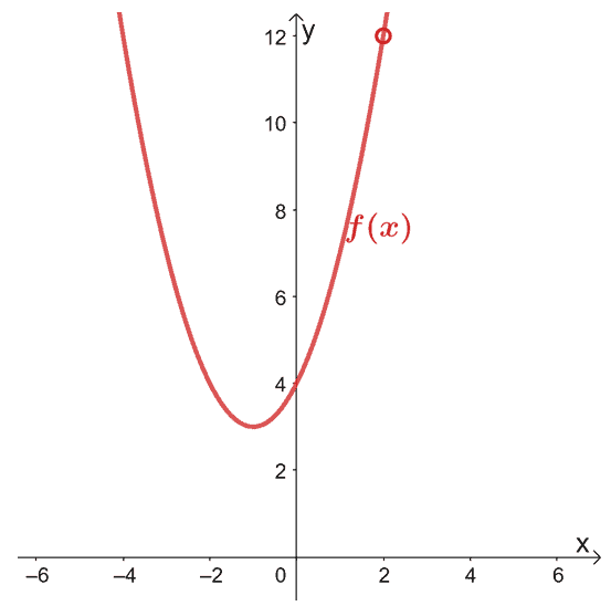
Determine the limit (if it exists) of the function as $x$ approaches the following:

a. $\lim_{x\rightarrow -1} f(x)$
b. $\lim_{x\rightarrow 0} f(x)$
c. $\lim_{x\rightarrow 2} f(x)$

2. Create a table of values (feel free to use a calculator) for the following functions, then approximate the limits of the functions to three decimal places.

a. $\lim_{x\rightarrow 0} \dfrac{1- e^{3x}}{x}$
b. $\lim_{x\rightarrow 0} (1+ 3x)^{\frac{1}{x}}$
c. $\lim_{x\rightarrow 25} \dfrac{5 – \sqrt{x}}{x – 25}$

3. Evaluate the limit (if it exists) of the following functions.
a. $\lim_{x\rightarrow -3} -\dfrac{x}{6}$
b. $\lim_{x\rightarrow 2} \dfrac{x – 2}{x^2 – 4}$
c. $\lim_{x\rightarrow 4} \dfrac{x^{3} – 64}{x – 4}$
d. $\lim_{x\rightarrow 0} \dfrac{\dfrac{1}{x + 5} – \dfrac{1}{5}}{x}$

4. Evaluate the limit (if it exists) of the following functions.
a. $\lim_{x\rightarrow -3} \dfrac{\dfrac{6}{x + 5}- 3}{x +3}$
b. $\lim_{x\rightarrow 0} \dfrac{\sqrt{9 + x} – 3}{x}$
c. $\lim_{x\rightarrow 0} \dfrac{1 – \cos 2x }{4x}$
d. $\lim_{x\rightarrow \infty} -\dfrac{2x^2 + 4x – 6}{(x – 3)^2}$

Answer Key

1.
a. $7$
b. $4$
c. $12$
2.
a. $-3$
b. $20.086$
c. $-0.100$
3.
a. $-\dfrac{1}{2}$
b. $\dfrac{1}{4}$
c. $48$
d. $-\dfrac{1}{25}$
4.
a. $-\dfrac{3}{2}$
b. $\dfrac{1}{6}$
c. $0$
d. $2$

Images/mathematical drawings are created with GeoGebra.