Line Integral – Definition, Properties, and Examples
Learning about the
line integral opens a wide range of functions that we can now study. In physics and engineering, we use line integrals to estimate the work of a particle in a force field or a mass in a gravitational field. Aside from its extensive applications, we can also establish generalized rules for the
fundamental theorem of calculus through line integrals – all the more reason why we need to be familiar with them.
Through line integrals, we can now integrate functions over any curve in the plane or space. This means that our integrand can now either be a scalar or vector field – opening a wide range of properties and techniques for us!Aside from its extensive applications, we can also establish generalized rules for the
fundamental theorem of calculus through line integrals – all the more reason why we need to be familiar with them.
What Is a Line Integral?
Line integrals allow us to integrate a wide range of functions including multivariable functions and vector fields. Simply put, the line integral is the
integral of a function that lies along a path or a curve.
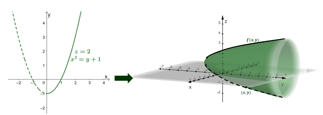
In our discussion of linear integrals, we’ll learn how to integrate linear functions that are part of a three-dimensional figure or
graphed on a vector field. We’ve learned how to integrate single and multivariable functions, so it’s time that we extend our knowledge to integrate parametric and vector functions.\begin{aligned} \textbf{Parametric Function: }&x = x(t), y = y(t), \phantom{xxd}a \leq t \leq b\\\\\textbf{Vector Function: }&\textbf{r}(t) = x(t)\textbf{i} + y(t)\textbf{j}, \phantom{xx}a \leq t \leq b \end{aligned}What makes these types of equations unique from the functions we’ve been working on so far? This time, we’re integrating over a curve (instead of an interval).

To establish the formal definition, let’s take a look at the smooth curve, $C$, as shown above. We’ve divided the curve into $n$ parts and it’s important to note that for line integrals, the distance in between is not necessarily equal. This means that $\{\Delta s_1, \Delta s_2, \Delta s_3, …, \Delta s_n \}$ will not have equal lengths unlike their single integral counterpart. However, the $x$-axis will remain partitioned and as we expand it and focus within the interval, the difference in between will be insignificant. We can add these segments and evaluate the limit of the sum similar to evaluating Riemann sums. This mental exercise leads us to understand the formal definition of line integrals.
Line Integral Definition
Suppose that $f$ is a function that is defined along the curve, $C$, we can write the line integral of the function in $\mathbb{R}^2$ or $\mathbb{R}^3$ as shown below.\begin{aligned} \textbf{Two-dimensional: }\int_{C} f(x, y) \phantom{x}ds &= \lim_{n \rightarrow \infty} \sum_{i = 1}^{n} f(x_i, y_i) \Delta s_i\\\textbf{Three-dimensional: }\int_{C} f(x, y, z) \phantom{x}ds &= \lim_{n \rightarrow \infty} \sum_{i = 1}^{n} f(x_i, y_i, z_i) \Delta s_i \end{aligned}Notice that we leave $ds$ as it is? This is to symbolize that we’re observing the line integral by tracing along the curve, $C$. In the past, we’ve been integrating along the $x$-axis (or with respect to $dx$) and the $y$-axis (or with respect to $dy$). This time, we’re integrating the function along an arc length.\begin{aligned}x &= x(t) \\ y&= y(t)\\ a\leq &t \leq b\end{aligned}Suppose that our curve, $C$, has the parametric equations shown above. Using our knowledge of
parametric curves, we can find the expression of the arc length, $L$, of $C$ as shown below.\begin{aligned}L &= \int_{a}^{b} \sqrt{\left(\dfrac{dx}{dt}\right)^2 + \left(\dfrac{dy}{dt}\right)^2} \phantom{x}dt\end{aligned}This means that we can rewrite our expression for line integrals both in the plane and in space using our parametric expressions for $ds$ and $f(x, y)$.
| Line Integral in Plane | \begin{aligned}\int_C f(x, y) \phantom{x}ds &= \int_{a}^{b}f(x(t), y(t))\sqrt{\left(\dfrac{dx}{dt} \right )^2+\left(\dfrac{dy}{dt} \right )^2 } \phantom{x}dt\end{aligned} |
| Line Integral in Space | \begin{aligned}\int_C f(x, y, z) \phantom{x}ds &= \int_{a}^{b}f(x(t), y(t), z(t))\sqrt{\left(\dfrac{dx}{dt} \right )^2+ \left(\dfrac{dy}{dt} \right )^2 +\left(\dfrac{dz}{dt} \right )^2 } \phantom{x}dt\end{aligned} |
This definition of line integrals works when we’re dealing with simple planes and parametric curves. Let’s now explore other forms of the line integral’s definition that will help us when evaluate line integrals of vector functions. As we have mentioned earlier, we can use line integrals on vector functions such as $\textbf{r}(t) = x(t) \textbf{i} + y(t) \textbf{j} + z(t) \textbf{k}$. In fact, we can use this expression to rewrite $s$ and $ds$ using vector components.
| LINE INTEGRAL IN VECTOR FUNCTIONSSuppose that we have $\textbf{r}(t)$ is a vector function, we can write its line integral over the curve, $C$, as shown below.\begin{aligned}\textbf{In two dimensions }&:\\ds &= \sqrt{x\prime(t)^2 + y\prime(t)^2}\\&= |\textbf{r}\prime(t)|\\\int_{a}^{b} f(x, y) \phantom{x}ds &= \int_{a}^{b} f(\textbf{r}(t))|\textbf{r}\prime(t)| \phantom{x}dt\\\\\textbf{In three dimensions }&:\\ds &= \sqrt{x\prime(t)^2 + y\prime(t)^2 + z\prime(t)^2}\\&= |\textbf{r}\prime(t)|\\\int_{a}^{b} f(x, y, z) \phantom{x}ds &= \int_{a}^{b} f(\textbf{r}(t))|\textbf{r}\prime(t)| \phantom{x}dt\end{aligned} |
Line Integral Properties
It is also important that we know the properties that apply to line integrals. There are instances when we’re asked to evaluate line integrals with respect to a differential instead of an arc length. When that happens, use the rules for integrating line integrals with respect to one variable as shown below.
| Line integral with respect to $\boldsymbol{x}$ | \begin{aligned}\int_{C} f(x, y)\phantom{x}dx &= \int_{a}^{b} f(x(t), y(t)) x\prime(t) \phantom{x}dt\end{aligned} |
| Line integral with respect to $\boldsymbol{y}$ | \begin{aligned}\int_{C} f(x, y)\phantom{x}dy &= \int_{a}^{b} f(x(t), y(t)) y\prime(t) \phantom{x}dt\end{aligned} |
This is why it’s important to identify whether you’re given $ds$, $dx$, $dy$, or even $dz$ for the differential. This normally occurs when working with line integrals with different differentials simultaneously. Here’s a helpful way to abbreviate these into a sum of two line integrals:\begin{aligned}\int_{C} P(x, y) \phantom{x}dy + Q(x, y) \phantom{x}dx &= \int_{C} P(x, y) \phantom{x}dy + \int_{C} Q(x, y) \phantom{x}dx \end{aligned}Aside from these notations, it’s important to account for the instances when the line integrals switch directions. Here are some important properties involving signs of line integrals.\begin{aligned}\int_{-C} f(x, y) \phantom{x}dx &= -\int_{C} f(x, y) \phantom{x}dx\\\int_{-C} f(x, y) \phantom{x}dy &= -\int_{C} f(x), y \phantom{x}dy\\\int_{-C} P \phantom{x}dx + Q \phantom{x}dy &= -\int_{C} P \phantom{x}dx + Q \phantom{x}dy\end{aligned}If you have noticed, we’ve been writing down properties in two-dimensions. This doesn’t mean that these properties do not apply to three-dimensional coordinate system. In fact, they do and you can write the properties down by extending the expressions to account for $z$.
| LINE INTEGRAL PROPERTIES in 3DSuppose that $C$ is a smooth curve parametrized by the following equations:\begin{aligned}x&= x(t)\\ y&= y(y)\\z &= z(t)\\ a \leq &t \leq b \end{aligned}The line integrals of $C$ will satisfy the following equations:\begin{aligned}\int_{C} f(x, y, z)\phantom{x}dx &= \int_{a}^{b} f(x(t), y(t), z(t)) x\prime(t) \phantom{x}dt\\\int_{C} f(x, y, z)\phantom{x}dy &= \int_{a}^{b} f(x(t), y(t), z(t)) y\prime(t) \phantom{x}dt\\\int_{C} f(x, y, z)\phantom{x}dz &= \int_{a}^{b} f(x(t), y(t), z(t)) z\prime(t) \phantom{x}dt\\\\\int_{C} P \phantom{x}dx + Q \phantom{x}dy + R \phantom{x}dz &= \int_{C} P(x, y, z) \phantom{x}dx + \int_{C} Q(x, y, z) \phantom{x}dy+ \int_{C} R(x, y, z) \phantom{x}dz\end{aligned} |
Now that we’ve established the fundamental definition and properties involving line integrals, it’s time that we understand the process of evaluating line integrals. By the end of the sections below, we’ll make sure that you also know how to apply the process in solving word problems that involve line integrals.
How To Evaluate Line Integrals?
For us to evaluate line integrals, it’s important that we make sure that we’ve parametrized the equations in terms of one variable. Once simplified, evaluate the new expression within the set limit of integrations for the curve and using the expression of the differential in terms of $t$.In case you need a refresher, head over to this
link. For now, let us show you the common parametric equations you might encounter:
| Cartesian Form | Parametric Form |
| \begin{aligned}x^2 + y^2 &= r^2\end{aligned} | Counter-clockwise Direction\begin{aligned}x&= r\cos t\\y&= r \sin t\\0 \leq &t \leq 2\pi\end{aligned} | Clockwise Direction\begin{aligned}x&= r\cos t\\y&= -r \sin t\\0 \leq &t \leq 2\pi\end{aligned} |
| \begin{aligned}\dfrac{x^2}{a^2} + \dfrac{y^2}{b^2} &= 1\end{aligned} | Counter-clockwise Direction\begin{aligned}x&= a\cos t\\y&= b \sin t\\0 \leq &t \leq 2\pi\end{aligned} | Clockwise Direction\begin{aligned}x&= a\cos t\\y&= -b \sin t\\0 \leq &t \leq 2\pi\end{aligned} |
| \begin{aligned}y&= f(x) \\x &= g(y) \end{aligned} | \begin{aligned}x&= t\\ y &= f(t) \end{aligned} | \begin{aligned}x&= g(t)\\ y &= t \end{aligned} |
Head over to this table in case you need a guide when parametrizing Cartesian functions to their parametric forms or in terms of $t$. This reduces the number of variables we need to work on – making the process of evaluating line integrals easier. Rewrite $ds$, $dx$, $dy$, or $dz$ in terms of $t$ as well. Once we have an integral expression all in terms of $t$, evaluate the resulting expression.The best way to understand the process is by working out on a specific line integral.\begin{aligned}\textbf{Line Integral: }&\int_{C} 2xy^4 \phantom{x}ds\\\textbf{Half Circle: }&x^2 + y^2 = 9 \end{aligned}For example, if we want to evaluate the line integral, $\int_{C} 2xy^4 \phantom{x}ds$, where our curve $C$ is a semicircle traced by the function, $x^2 + y^2 = 9$, and in a counter-clockwise direction and at the left of the $y$-axis.

\begin{aligned} x&= r \cos t\\ y&= r \sin t\end{aligned}Rewrite the curve, $x^2 +y^2 =9$ in its parametric form using the equations shown above. The semicircle has a radius of $3$ units, so $r = 3$.\begin{aligned} x&= 3 \cos t\\ y&= 3 \sin t\end{aligned}The semicircle is lying above the $x$-axis, so the limits of integration for our line integral is $\dfrac{\pi}{2} \leq t \leq \dfrac{3\pi}{2} $. Now, let’s find the expression for $ds$ by taking the derivatives of $x(t)$ and $y(t)$.
| \begin{aligned}\boldsymbol{\dfrac{dx}{dt}}\end{aligned} | \begin{aligned}\boldsymbol{\dfrac{dy}{dt}}\end{aligned} |
| \begin{aligned}x(t) &= 3\cos t\\\dfrac{dx}{dt} &= -3 \sin t \end{aligned} | \begin{aligned}y(t) &= 3\sin t\\\dfrac{dy}{dt} &= 3 \cos t \end{aligned} |
| \begin{aligned}ds &= \sqrt{\left(\dfrac{dx}{dt} \right )^2 + \left(\dfrac{dy}{dt} \right )^2} \phantom{x}dt\\&= \sqrt{(-3 \sin t)^2 + (3 \cos t)^2} \phantom{x}dt\\&= \sqrt{3^2(\sin^2 t + \cos^2 t)}\phantom{x}dt\\&= 3 \phantom{x}dt\end{aligned} |
Now that we have all the components of our line integral in terms of $t$, we can go ahead and evaluate the line integral.\begin{aligned}\int_{C} 2xy^4 \phantom{x}ds &= \int_{\pi/2}^{3\pi/2} 2(3 \cos t)(3 \sin t)^4 \cdot 3 \phantom{x}dt\\&= 2(3^6)\int_{\pi/2}^{3\pi/2} \cos t \sin^4 t \phantom{x}dt\\&= 1458\left[\dfrac{\sin^5 t}{5} \right ]_{\pi/2}^{3\pi/2}\\&= \dfrac{1458}{5} \left(\sin^5 \dfrac{3\pi}{2} – \sin^5 \dfrac{\pi}{2} \right )\\&= \dfrac{2916}{5} \end{aligned}This means that the line integral is equal to $\dfrac{2916}{5}$ or $583.2$. Apply a similar process when evaluating a line integral over a curve $C$. Now, let’s see how we can evaluate the line integrals given two points of a line segment.
How To Do a Line Integral of a Segment?
When given $\int_{C} f(x,y) \phantom{x}ds$, we can integrate the line integral by parametrizing the line segment’s expression in terms of $t$. In the past, we’ve learned how to parametrize equations given two points. In case you need a refresher, review the equations shown below.\begin{aligned}\textbf{r}(t) &= (1 – t)<x_o, y_o, z_o> + t<x_1, y_1, z_1>\\x &= (1 – t)x_o + tx_1 \\y &= (1 – t)y_o + ty_1\\z &= (1 – t)z_o + tz_1 \\0 &\leq t \leq 1\end{aligned}This parametrization works when we’re given the points, $(x_o, y_o, z_o)$ and $(x_1, y_1, z_1)$, that the line segment passes through.\begin{aligned}\int_{C} &2x^4 \phantom{x}ds\\\text{from } (-1&, 1)\text{ to } (2, 4)\end{aligned}Let’s try to evaluate the line integral, $\int_{C} 2x^4 \phantom{x}ds$, where $C$ represents the line segment that passes through the points, $(-1, 1)$ and $(2, 4)$. Let’s use the formula for $\textbf{r}(t)$, as shown above. Use $(x_o, y_o) = (-1, 1)$ and $(x_1, y_1) = (2, 4)$.\begin{aligned}\textbf{r}(t) &= (1 – t)<-1, 4> + t<2, 4>\\&= <-1(1- t), 4(1 -t)> + <2t, 4t>\\&=<-1+ t, 4 – 4t> +<2t, 4t>\\&= <-1+ 3t, 4>\\\\x&= -1 + 3t, y= 4\end{aligned}Recall that this parametrization works when $t$ satisfies the inequality, $0 \leq t\leq 1$, so we now have a limit of integration. Since we have $x = -1 + 3t$ and $y = 4$, we can rewrite $ds$ in terms of $t$.\begin{aligned}\dfrac{dx}{dt} &= 3, \dfrac{dy}{dt} =0\\ds &= \sqrt{\left(\dfrac{dx}{dt} \right )^2+ \left(\dfrac{dy}{dt} \right )^2}\phantom{x}dt\\&= \sqrt{9} \phantom{x}dt\\&= 3\phantom{x} dt\end{aligned}Rewrite the expression for $x$, $y$, and $ds$ in terms of $t$ then evaluate the resulting integral.\begin{aligned}\int_{C} 2x^4 \phantom{x}ds &= \int_{0}^{1} 2(-1 + 3t)^4 \cdot 3\phantom{x}dt\\&= 2\int_{0}^{1} 3(-1+ 3t)^4 \phantom{x}dt\\&= 2\cdot \dfrac{1}{5}[(-1 + 3t)^5]_0^{1}\\&= \dfrac{2}{5}[(-1 + 3)^5 – (-1 + 0)^5]\\&= \dfrac{2}{5}(32 + 1)\\&= \dfrac{66}{5}\end{aligned}Hence, we’ve shown you how to evaluate line integrals when given the points that a line segment passes through. We’ve prepared more examples for you to work on and we’ll show you how to apply these concepts to solve word problems involving line integrals.
Example 1Evaluate the line integral, $\int_{C} 2x \phantom{x}ds$, over the following curves.a. $C_1$: $y = x^2$, where $x$ is within the interval, $[-2, 2]$
b. $C_2$: The line segment that passes through the points, $(-2,2)$ and $(2, 2)$.
c. $C_3$: The line segment that passes through the points, $(2,2)$ and $(-2, 2)$.
SolutionThis example highlights how the values of the line integrals vary depending on the curve that the function is integrated over. Here’s the graph of the curve for our first item, $C_1$: $y=x^2$.

To evaluate the expression for $\int_{C_1} 2x \phantom{x}ds$, we begin by parameterizing the equations representing $C_1$.\begin{aligned}x&= t\\y&= t^2\\-2 \leq &t\leq 2\end{aligned}Rewrite the expression for $ds$ by using the derivatives of $x(t)$ and $y(t)$ as shown below.\begin{aligned}\dfrac{dx}{dt} &= 1, \dfrac{dy}{dt} =2t\\ds &= \sqrt{\left(\dfrac{dx}{dt} \right )^2+ \left(\dfrac{dy}{dt} \right )^2}\phantom{x}dt\\&= \sqrt{1 + 4t^2} \phantom{x}dt\end{aligned}Now that we have rewritten all the key components in terms of $t$, let’s go ahead and rewrite the line integral and evaluate the resulting expression.\begin{aligned}\int_{C_1} 2x \phantom{x}ds &= \int_{-2}^{2} 2(t) \cdot \sqrt{1 +4t^2} \phantom{x}dt\\&= 2\int_{-2}^{2} t\sqrt{1 +4t^2} \phantom{x}dt\\&= 2\cdot \dfrac{1}{12} \left[(1 + 4t^2)^{3/2} \right ]_{-2}^{2}\\&= \dfrac{1}{6}\left[(17)^{3/2} -(17)^{3/2} \right ]\\&= 0\end{aligned}a. This means that $\int_{C} 2x \phantom{x}ds$ is equal to $0$ when $C$ is a parabola defined by the equation, $y= x^2$.Now, let’s work on the second condition: finding the line integral’s value when the curve is a line segment that passes through $(-2,2)$ and $(2, 2)$. We begin by finding the parametric equation representing the line segment.\begin{aligned}\textbf{r}(t) &= (1 – t)<-2, 2> + t<2, 2>\\&= <-2(1- t), 2(1 -t)> + <2t, 2t>\\&=<-2+ 2t, 2 – 2t> +<2t, 2t>\\&= <-2+ 4t, 2>\\\\x&= -2 + 4t, y= 2\end{aligned}This parametric equation is only true when $0 \leq t \leq 1$. This also means that $\dfrac{dx}{dt} = 4$ and $\dfrac{dy}{dt} = 0$, so rewrite $ds$ in terms of $t$.\begin{aligned}ds &= \sqrt{\left(\dfrac{dx}{dt} \right )^2+ \left(\dfrac{dx}{dt} \right )^2}\phantom{x}dt\\&= \sqrt{16} \phantom{x}dt\\&= 4\phantom{x} dt\end{aligned}We now have all the key components to rewrite the line integral going over $C_2$.\begin{aligned}\int_{C_2} 2x \phantom{x}ds &= \int_{0}^{1} 2(-2 + 4t) \cdot 4 \phantom{x}dt\\&= -16\int_{0}^{1} (1 – 2t) \phantom{x}dt\\&= -16[t – t^2]_{0}^{1}\\&= -16[(1 – 1) – 0]\\&= 0\end{aligned}Hence, $\int_{C_2} 2x \phantom{x}ds = 0$. Let us show you a simpler approach to this problem – by observing the points where the line segment passes through $(-2, 2)$ and $(2, 2)$. This means that the Cartesian form of the equation representing the line segment is $y =2$.\begin{aligned}x&= t\\ y&= 2\\ds &= \sqrt{1}\phantom{x}dt\\ -2\leq &t \leq 2\end{aligned}Use these expressions to evaluate the line integral over the line segment, $C_2$.\begin{aligned}\int_{C_2} 2x \phantom{x}ds &= \int_{-2}^{2} 2t \sqrt{1}\phantom{x}dt\\&= 2\int_{-2}^{2} t\phantom{x}dt\\&= [t^2]_{-2}^{2}\\&= (2)^2 -(-2)^2\\&= 0\end{aligned}This is a good example highlighting that there are instances when observing the line segment’s Cartesian form helps before we use $\textbf{r}(t) = (1- t)<x_o, y_o> + t<x_1, y_1>$.b. This shows that by using either of the two methods, we should still have $\int_{C_2} 2x \phantom{x}ds = 0$.The line segment for the third item actually has the same form with $C_2$. The only difference is that the direction is reversed, so we expect $C_3$ to be the negative counterpart of $C_2$.\begin{aligned}C_3 &= -C_2\end{aligned}This means that the line integral will also be equal to zero. We can confirm this by evaluating the line integral. For the sake of discussion, let us parametrize $C_3$.\begin{aligned}\textbf{r}(t) &= (1 – t)<2, 2> + t<-2, 2>\\&= <2(1- t), 2(1 -t)> + <-2t, 2t>\\&=<2 – 2t, 2 – 2t> +<-2t, 2t>\\&= <2 – 4t, 2>\end{aligned}Now, evaluate the line integral similar to our previous example and this shows that $\int_{C_3} 2x \phantom{x}ds$ is equal to zero.\begin{aligned}\int_{C_3} 2x \phantom{x}ds &= \int_{0}^{1} 2(2 – 4t) \cdot 4 \phantom{x}dt\\&= 16\int_{0}^{1} (1 – 2t) \phantom{x}dt\\&= 16[t – t^2]_{0}^{1}\\&= 0\end{aligned}
Example 2Evaluate the line integral, $\int_{C} xyz \phantom{x}ds$, where the curve, $C$, is represented by the vector function, $\textbf{r}(t) = <\cos t, \sin t, 4t>$, where $0 \leq t \leq 4\pi$.
SolutionWe’ve encountered our first helix when we studied vector functions. Here’s the graph of the helix represented by the vector function, $\textbf{r}(t) = <\cos t, \sin t, 4t>$, where $0 \leq t \leq 4\pi$.

Since we have the $x$, $y$, and $z$ components already in terms of $t$, we can go ahead and find the expression for $ds$.
| \begin{aligned}x &= \cos t\\\dfrac{dx}{dt} &= -\sin t\end{aligned} | \begin{aligned}y &= \sin t\\\dfrac{dx}{dt} &= \cos t\end{aligned} | \begin{aligned}z &= 4t\\\dfrac{dz}{dt} &= 4\end{aligned} |
| \begin{aligned}ds &= \sqrt{\left(\dfrac{dx}{dt} \right )^2+ \left(\dfrac{dy}{dt} \right )^2+ \left(\dfrac{dz}{dt} \right )^2}\phantom{x}dt\\&= \sqrt{\cos^2 t + \sin^2 t+ 4^2} \phantom{x}dt\\&= \sqrt{1 + 16} \phantom{x}dt\\&= \sqrt{17} \phantom{x}dt\end{aligned} |
Now that we have all the key components, let’s rewrite the line integral all in terms of $t$ then evaluate the resulting expression using
integration by parts.\begin{aligned}\int_{C} xyz \phantom{x}ds &= \int_{0}^{4\pi} (\cos t)(\sin t)(4t) \cdot \sqrt{17}\phantom{x} dt\\&= 4\sqrt{17}\int_{0}^{4\pi}t\cos t\sin t \phantom{x}dt\\&= 4\sqrt{17}\int_{0}^{4\pi} \dfrac{t}{2}\sin 2t \phantom{x}dt\\&= \dfrac{4\sqrt{17}}{2}\int_{0}^{4\pi} t\sin 2t \phantom{x}dt\\&= \dfrac{4\sqrt{17}}{2} \left[\dfrac{1}{4}\sin \left(2t\right) – \dfrac{1}{2}t\cos \left(2t\right)\right ]_{0}^{4\pi}\\&= \dfrac{4\sqrt{17}}{2}(-2\pi – 0)\\&= -4\sqrt{17}\pi\end{aligned}Hence, $\int_{C} xyz \phantom{x}ds$ is equal to $-4\sqrt{17}$ or approximately equal to $-51.81$.
Example 3Evaluate the line integral, $\int_{C} \cos \pi y \phantom{x}dy + 2xy^2 \phantom{x}dx$, where the curve, $C$, is the line segment that passes through the points, $(1, 3)$ and $(-2, 0)$.
SolutionAs with our previous examples, when parametrizing a line segment, we use the parametric equation, $\textbf{r}(t) = (1 –t)<x_o, y_o > + t<x_1, y_1>$, where $0\leq t\leq 1$.\begin{aligned}\textbf{r}(t) &= (1- t)<1, 3> + t<-2, 0>\\&= <(1- t), 3(1 -t)> +<-2t, 0>\\&= <1 – 3t, 3 – 3t>\end{aligned}Use the general form of line integrals to rewrite $\int_{C} \cos \pi y \phantom{x}dy + 2xy^2 \phantom{x}dx$.\begin{aligned}\int_{C} P(x, y) \phantom{x}dy + Q(x, y) \phantom{x}dx &= \int_{C} P(x, y) \phantom{x}dy + \int_{C} Q(x, y) \phantom{x}dx\\\int_{C} \cos \pi y \phantom{x}dy + 2xy^2 \phantom{x}dx &=\int_{C} \cos \pi y \phantom{x}dy +\int_{C} 2xy^2 \phantom{x}dx \end{aligned}By rewriting the line integral this way, we can rewrite each sub line integral’s components in terms of $t$. Using $x = 1 – 3t$ and $y =3 – 3t $, rewrite $\int_{C} \cos \pi y \phantom{x}dy$ and $+\int_{C} 2xy^2 \phantom{x}dx$ then evaluate the resulting expressions.
| \begin{aligned}\boldsymbol{\int_{C} f(x, y)\phantom{x}dx = \int_{a}^{b} f(x(t), y(t)) x\prime(t) \phantom{x}dt}\end{aligned} | \begin{aligned}\boldsymbol{\int_{C} f(x, y)\phantom{x}dy = \int_{a}^{b} f(x(t), y(t)) y\prime(t) \phantom{x}dt}\end{aligned} |
| \begin{aligned}\int_{C} 2xy^2 \phantom{x}dx &= \int_{0}^{1} 2(1 – 3t)(3 – 3t)^2 \cdot x^\prime(t) \phantom{x}dt\\&= 2\int_{0}^{1} (1 -3t)(3 -3t)^2 \cdot -3\phantom{x}dt\\&= -6\int_{0}^{1} -27t^3+ 63t^2- 45t+ 9 dt\\&= -6\left[-\dfrac{27t^4}{4} + 21t^3 -\dfrac{45t^2}{2} + 9t \right ]_{0}^{1}\\&= -6\left(\dfrac{3}{4}\right)\\&= -\dfrac{9}{2} \end{aligned} | \begin{aligned}\int_{C} \cos \pi y \phantom{x}dy &= \int_{0}^{1} \cos \pi(3 – 3t) \cdot y^\prime(t) \phantom{x}dt\\&=\int_{0}^{1} \cos \pi(3 – 3t) \cdot -3 \phantom{x}dt\\&= -3\left[-\dfrac{1}{3\pi}\sin(3\pi – 3\pi t) \right ]_{0}^{1}\\&= \dfrac{1}{\pi}(\sin 0 – \sin 3\pi)\\&=0 \end{aligned} |
Now that we’ve evaluated the values of the two line integrals, so combine these two to find $\int_{C} \cos \pi y \phantom{x}dy + 2xy^2 \phantom{x}dx$’s value.\begin{aligned}\int_{C} \cos \pi y \phantom{x}dy + 2xy^2 \phantom{x}dx &=\int_{C} \cos \pi y \phantom{x}dy +\int_{C} 2xy^2 \phantom{x}dx\\&= 0 -\dfrac{9}{2}\\&= -\dfrac{9}{2} \end{aligned}
Practice Questions
1. Evaluate the line integral, $\int_{C} 4x \phantom{x}ds$, over the following curves.
a. $C_1$: $y = 3x^2$, where $x$ is within the interval, $[-4, 4]$
b. $C_2$: The line segment that passes through the points, $(-4, 4)$ and $(4, 4)$.
c. $C_3$: The line segment that passes through the points, $(4, 4)$ and $(-4, 4)$.
2. Evaluate the line integral, $\int_{C} xyz \phantom{x}ds$, where the curve, $C$, is represented by the vector function, $\textbf{r}(t) = <\cos t, \sin t, 5t>$, where $0 \leq t \leq 6\pi$.
3. Evaluate the line integral, $\int_{C} \sin \pi y \phantom{x}dy + xy^2 \phantom{x}dx$, where the curve, $C$, is the line segment that passes through the points, $(1, 2)$ and $(-1, 1)$.
4. A particle is moving along the line segment that passes through the points,from $(0, 5, 1)$ to $(1, 4, 2)$. What is the work done by the particle on a vector field, $\textbf{V}(x, y,z) = <x, 3xy, -x –z>$? (Here’s a hint: $\text{Work} = \int_{C} F \cdot r$)
Answer Key
1. $\int_{C_1} 4x \phantom{x}ds = \int_{C_2} 4x \phantom{x}ds =\int_{C_3} 4x \phantom{x}ds$
2.
$\begin{aligned}\int_{C} xyz \phantom{x}ds &= 5\sqrt{26} \int_{0}^{6\pi} t \cos t \sin t \phantom{x}dt\\&= -\dfrac{15\sqrt{26}\pi}{2}\\&\approx -120.14 \end{aligned}$
3.
$\begin{aligned}\int_{C} \sin \pi y \phantom{x}dy + xy^2 \phantom{x}dx &= -\int_{0}^{1} \sin \pi(2 –t) \phantom{x}dt – 2\int_{0}^{1} (1- 2t)(2 –t)^2 \phantom{x}dt\\&= 0 – 1\\&= -1\end{aligned}$4. The work done by the particle is $8$ units.
Images/mathematical drawings are created with GeoGebra.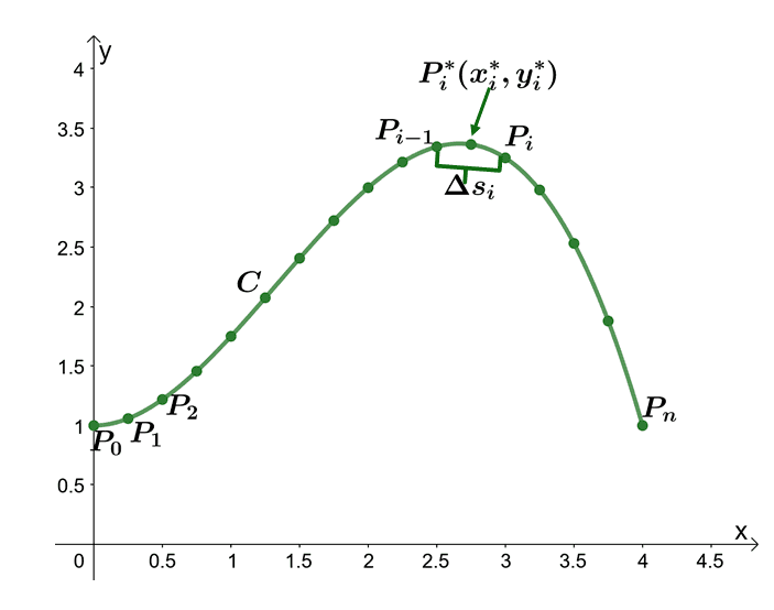 To establish the formal definition, let’s take a look at the smooth curve, $C$, as shown above. We’ve divided the curve into $n$ parts and it’s important to note that for line integrals, the distance in between is not necessarily equal. This means that $\{\Delta s_1, \Delta s_2, \Delta s_3, …, \Delta s_n \}$ will not have equal lengths unlike their single integral counterpart. However, the $x$-axis will remain partitioned and as we expand it and focus within the interval, the difference in between will be insignificant. We can add these segments and evaluate the limit of the sum similar to evaluating Riemann sums. This mental exercise leads us to understand the formal definition of line integrals.
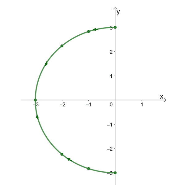 \begin{aligned} x&= r \cos t\\ y&= r \sin t\end{aligned}Rewrite the curve, $x^2 +y^2 =9$ in its parametric form using the equations shown above. The semicircle has a radius of $3$ units, so $r = 3$.\begin{aligned} x&= 3 \cos t\\ y&= 3 \sin t\end{aligned}The semicircle is lying above the $x$-axis, so the limits of integration for our line integral is $\dfrac{\pi}{2} \leq t \leq \dfrac{3\pi}{2} $. Now, let’s find the expression for $ds$ by taking the derivatives of $x(t)$ and $y(t)$.
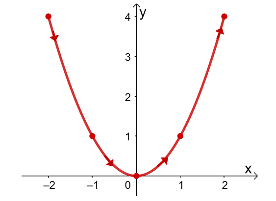 To evaluate the expression for $\int_{C_1} 2x \phantom{x}ds$, we begin by parameterizing the equations representing $C_1$.\begin{aligned}x&= t\\y&= t^2\\-2 \leq &t\leq 2\end{aligned}Rewrite the expression for $ds$ by using the derivatives of $x(t)$ and $y(t)$ as shown below.\begin{aligned}\dfrac{dx}{dt} &= 1, \dfrac{dy}{dt} =2t\\ds &= \sqrt{\left(\dfrac{dx}{dt} \right )^2+ \left(\dfrac{dy}{dt} \right )^2}\phantom{x}dt\\&= \sqrt{1 + 4t^2} \phantom{x}dt\end{aligned}Now that we have rewritten all the key components in terms of $t$, let’s go ahead and rewrite the line integral and evaluate the resulting expression.\begin{aligned}\int_{C_1} 2x \phantom{x}ds &= \int_{-2}^{2} 2(t) \cdot \sqrt{1 +4t^2} \phantom{x}dt\\&= 2\int_{-2}^{2} t\sqrt{1 +4t^2} \phantom{x}dt\\&= 2\cdot \dfrac{1}{12} \left[(1 + 4t^2)^{3/2} \right ]_{-2}^{2}\\&= \dfrac{1}{6}\left[(17)^{3/2} -(17)^{3/2} \right ]\\&= 0\end{aligned}a. This means that $\int_{C} 2x \phantom{x}ds$ is equal to $0$ when $C$ is a parabola defined by the equation, $y= x^2$.Now, let’s work on the second condition: finding the line integral’s value when the curve is a line segment that passes through $(-2,2)$ and $(2, 2)$. We begin by finding the parametric equation representing the line segment.\begin{aligned}\textbf{r}(t) &= (1 – t)<-2, 2> + t<2, 2>\\&= <-2(1- t), 2(1 -t)> + <2t, 2t>\\&=<-2+ 2t, 2 – 2t> +<2t, 2t>\\&= <-2+ 4t, 2>\\\\x&= -2 + 4t, y= 2\end{aligned}This parametric equation is only true when $0 \leq t \leq 1$. This also means that $\dfrac{dx}{dt} = 4$ and $\dfrac{dy}{dt} = 0$, so rewrite $ds$ in terms of $t$.\begin{aligned}ds &= \sqrt{\left(\dfrac{dx}{dt} \right )^2+ \left(\dfrac{dx}{dt} \right )^2}\phantom{x}dt\\&= \sqrt{16} \phantom{x}dt\\&= 4\phantom{x} dt\end{aligned}We now have all the key components to rewrite the line integral going over $C_2$.\begin{aligned}\int_{C_2} 2x \phantom{x}ds &= \int_{0}^{1} 2(-2 + 4t) \cdot 4 \phantom{x}dt\\&= -16\int_{0}^{1} (1 – 2t) \phantom{x}dt\\&= -16[t – t^2]_{0}^{1}\\&= -16[(1 – 1) – 0]\\&= 0\end{aligned}Hence, $\int_{C_2} 2x \phantom{x}ds = 0$. Let us show you a simpler approach to this problem – by observing the points where the line segment passes through $(-2, 2)$ and $(2, 2)$. This means that the Cartesian form of the equation representing the line segment is $y =2$.\begin{aligned}x&= t\\ y&= 2\\ds &= \sqrt{1}\phantom{x}dt\\ -2\leq &t \leq 2\end{aligned}Use these expressions to evaluate the line integral over the line segment, $C_2$.\begin{aligned}\int_{C_2} 2x \phantom{x}ds &= \int_{-2}^{2} 2t \sqrt{1}\phantom{x}dt\\&= 2\int_{-2}^{2} t\phantom{x}dt\\&= [t^2]_{-2}^{2}\\&= (2)^2 -(-2)^2\\&= 0\end{aligned}This is a good example highlighting that there are instances when observing the line segment’s Cartesian form helps before we use $\textbf{r}(t) = (1- t)<x_o, y_o> + t<x_1, y_1>$.b. This shows that by using either of the two methods, we should still have $\int_{C_2} 2x \phantom{x}ds = 0$.The line segment for the third item actually has the same form with $C_2$. The only difference is that the direction is reversed, so we expect $C_3$ to be the negative counterpart of $C_2$.\begin{aligned}C_3 &= -C_2\end{aligned}This means that the line integral will also be equal to zero. We can confirm this by evaluating the line integral. For the sake of discussion, let us parametrize $C_3$.\begin{aligned}\textbf{r}(t) &= (1 – t)<2, 2> + t<-2, 2>\\&= <2(1- t), 2(1 -t)> + <-2t, 2t>\\&=<2 – 2t, 2 – 2t> +<-2t, 2t>\\&= <2 – 4t, 2>\end{aligned}Now, evaluate the line integral similar to our previous example and this shows that $\int_{C_3} 2x \phantom{x}ds$ is equal to zero.\begin{aligned}\int_{C_3} 2x \phantom{x}ds &= \int_{0}^{1} 2(2 – 4t) \cdot 4 \phantom{x}dt\\&= 16\int_{0}^{1} (1 – 2t) \phantom{x}dt\\&= 16[t – t^2]_{0}^{1}\\&= 0\end{aligned}Example 2Evaluate the line integral, $\int_{C} xyz \phantom{x}ds$, where the curve, $C$, is represented by the vector function, $\textbf{r}(t) = <\cos t, \sin t, 4t>$, where $0 \leq t \leq 4\pi$.SolutionWe’ve encountered our first helix when we studied vector functions. Here’s the graph of the helix represented by the vector function, $\textbf{r}(t) = <\cos t, \sin t, 4t>$, where $0 \leq t \leq 4\pi$.
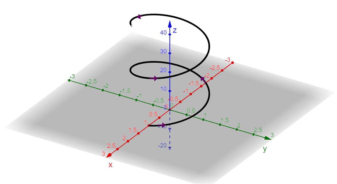 Since we have the $x$, $y$, and $z$ components already in terms of $t$, we can go ahead and find the expression for $ds$.