JUMP TO TOPIC
Logistic Equation – Explanation & Examples
 The definition of the logistic equation is:
“The logistic equation is a sigmoid function, which takes any real number and outputs a value between zero and certain positive number.”
In this topic, we will discuss the logistic equation from the following aspects:
- What is the logistic equation?
- Logistic equation formula.
- How to solve the logistic equation?
- Application of logistic function in ecology.
- Application of logistic function in statistics.
- Practice questions.
- Answer key.
1. What is the logistic equation?
The logistic equation is a sigmoid function, which takes any real number from negative infinity -∞ to positive infinity +∞ and outputs a value between zero and a certain positive number.
Logistic equation formula
The equation is :
f(x)=L/(1+e^(-k(x-x_0)) )
where:
f(x) is the logistic equation or function.
L is the logistic function or curve maximum value.
e is a mathematical constant approximately equal to 2.71828.
k is the logistic growth rate or steepness of the curve.
x_0 is the value of x at the sigmoid curve midpoint.
For values of x between -∞ to +∞, the logistic equation draws an S-curve with the curve f(x) approaching L as x approaches +∞ and approaching zero as x approaches -∞.
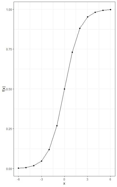
– Example 1
For the x values:
-6, -5, -4, -3, -2, -1, 0, 1, 2, 3, 4, 5, 6.
Draw the logistic curve when L = 1, k = 1, and x_0=0.
We follow these steps:
1. plot a table of values.
x |
-6 |
-5 |
-4 |
-3 |
-2 |
-1 |
0 |
1 |
2 |
3 |
4 |
5 |
6 |
2. Using the above formula, calculate the logistic function for each value.
x | f(x) |
| -6 | 0.002472623 |
-5 | 0.006692851 |
| -4 | 0.017986210 |
-3 | 0.047425873 |
-2 | 0.119202922 |
| -1 | 0.268941421 |
0 | 0.500000000 |
1 | 0.731058579 |
2 | 0.880797078 |
| 3 | 0.952574127 |
4 | 0.982013790 |
| 5 | 0.993307149 |
6 | 0.997527377 |
3. Plot the x values on the x-axis and the logistic function value on the y-axis.
Connect the intersecting points with a line to draw the sigmoid curve.
For comparison, we can add two other equations with the same parameters except that L = 5 and L =10 respectively.
We update the table.
x | f(x)_1 | f(x)_5 | f(x)_10 |
| -6 | 0.002472623 | 0.01236312 | 0.02472623 |
-5 | 0.006692851 | 0.03346425 | 0.06692851 |
| -4 | 0.017986210 | 0.08993105 | 0.17986210 |
-3 | 0.047425873 | 0.23712937 | 0.47425873 |
-2 | 0.119202922 | 0.59601461 | 1.19202922 |
| -1 | 0.268941421 | 1.34470711 | 2.68941421 |
0 | 0.500000000 | 2.50000000 | 5.00000000 |
1 | 0.731058579 | 3.65529289 | 7.31058579 |
| 2 | 0.880797078 | 4.40398539 | 8.80797078 |
3 | 0.952574127 | 4.76287063 | 9.52574127 |
| 4 | 0.982013790 | 4.91006895 | 9.82013790 |
5 | 0.993307149 | 4.96653575 | 9.93307149 |
| 6 | 0.997527377 | 4.98763688 | 9.97527377 |
Where f(x)_1 is the logistic function with L = 1, f(x)_5 is the logistic function with L = 5, and f(x)_10 is the logistic function with L = 10.
and plot the 3 different sigmoid curves.
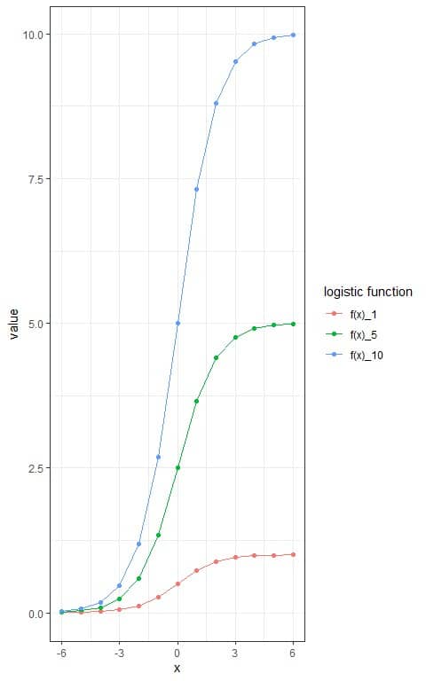
We see that the maximum of each logistic function is its L value.
– Example 2
For the x values:
-6, -5, -4, -3, -2, -1, 0, 1, 2, 3, 4, 5, 6.
Draw the logistic curve when L = 1, k = 1, 2, or 3, and x_0=0.
We follow these steps:
1. plot a table of values.
x |
-6 |
-5 |
-4 |
-3 |
-2 |
-1 |
0 |
1 |
2 |
3 |
4 |
5 |
6 |
2. Using the above formula, calculate the logistic function for each value and each k value.
We add 3 other columns, one for each logistic function.
x | f(x)_1 | f(x)_2 | f(x)_3 |
| -6 | 0.002472623 | 6.144175e-06 | 1.522998e-08 |
-5 | 0.006692851 | 4.539787e-05 | 3.059022e-07 |
| -4 | 0.017986210 | 3.353501e-04 | 6.144175e-06 |
-3 | 0.047425873 | 2.472623e-03 | 1.233946e-04 |
-2 | 0.119202922 | 1.798621e-02 | 2.472623e-03 |
| -1 | 0.268941421 | 1.192029e-01 | 4.742587e-02 |
0 | 0.500000000 | 5.000000e-01 | 5.000000e-01 |
1 | 0.731058579 | 8.807971e-01 | 9.525741e-01 |
| 2 | 0.880797078 | 9.820138e-01 | 9.975274e-01 |
3 | 0.952574127 | 9.975274e-01 | 9.998766e-01 |
4 | 0.982013790 | 9.996646e-01 | 9.999939e-01 |
| 5 | 0.993307149 | 9.999546e-01 | 9.999997e-01 |
6 | 0.997527377 | 9.999939e-01 | 1.000000e+00 |
Where f(x)_1 is the logistic function with k = 1, f(x)_2 is the logistic function with L = 2, and f(x)_3 is the logistic function with L = 3.
and plot the 3 different sigmoid curves.
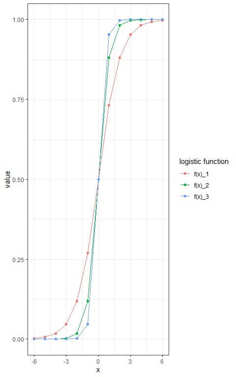 With increasing the k value, the sigmoid curve becomes steeper in its growth.
2. How to solve the logistic equation?
The logistic function finds applications in many fields, including ecology, chemistry, economics, sociology, political science, linguistics, and statistics.
We will focus on the application and the solving of logistic function in ecology and statistics.
– Application of logistic function in ecology
A typical application of the logistic equation is to model population growth, where the rate of reproduction is proportional to both the existing population and the amount of available resources.
The logistic differential equation for the population growth is:
dP/dt=rP(1-P/K)
Where:
P is the population size.
t is the time. The units of time can be hours, days, weeks, months, or years.
dP/dt is the instantaneous rate of change of the population as a function of time.
r is the growth rate.
K is the carrying capacity. The carrying capacity of an organism in a given environment is defined to be the maximum population of that organism that the environment can sustain indefinitely. It has the same unit as the population size.
The population growth rate changes over time. Biologists have found that in many biological systems, the population grows until a certain steady-state population is reached.
The concept of carrying capacity allows for the possibility that in a given area, only a certain number of a given organism or animal can thrive without running into resource issues.
Suppose that the initial population is small relative to the carrying capacity. Then P/K is small, possibly close to zero. Thus, the quantity in parentheses on the right-hand side of the logistic equation is close to 1, and the right-hand side of this equation is close to rP. The value of the rate r represents the proportional increase of the population P in one unit of time. So, the population grows rapidly.
However, as the population grows, some members of the population interfere with each other by competing for some critical resource, such as food or living space. The ratio P/K also grows, because K is constant. If the population remains below the carrying capacity, then P/K is less than 1, so 1-(P/K)>0 but less than 1. Therefore the growth rate decreases as a result.
If P=K then the right-hand side is equal to zero, and the population does not change (this is called maturity of the population).
The solution to the equation, with P_0 being the initial population is:
P(t)=K/(1+((K-P_0)/P_0 )e^(-rt) )
Note that K is the limiting value of P:
If the P_0 < K, then population grows till reaching K.
If P_0 >K, then population decreases till approach K.
– Example 1
A population of rabbits in a meadow is observed to be 200 rabbits at time t=0. Using an initial population of 200 and a growth rate of 0.04 per month, with a carrying capacity of 750 rabbits.
Draw the logistic curve of growth for this population.
We follow these steps:
1. The growth rate is per month so the x-axis will be in months. The 0 value will represent the current month, and 1 is the next month, and so on.
We can also plot negative values on the x-axis to represent the previous month and so on.
In a table, we write the next 12 values (next year) and the previous 12 values (previous year).
So the x values will range from -12 to 12.
In a table:
t_months |
-12 |
-11 |
-10 |
-9 |
-8 |
-7 |
-6 |
-5 |
-4 |
-3 |
-2 |
-1 |
0 |
1 |
2 |
3 |
4 |
5 |
6 |
7 |
8 |
9 |
10 |
11 |
12 |
2. We know that the population at the current month or t = 0 is 200. We use the above equation to know the population size for all these months:
P(t)=K/(1+((K-P_0)/P_0 )e^(-rt) )=750/(1+((750-200)/200)e^(-0.04t) )
For example, at time = 0:
The population size at time = 0 = P(0) = 750/1+(750-200/200)Xe^(-0.04X0) = 750/(1+((750-200)/200))= 200.
Using the above formula, calculate the population size for each time value and update the table.
t_months | population |
-12 | 137.7612 |
-11 | 142.3165 |
-10 | 146.9863 |
| -9 | 151.7710 |
-8 | 156.6710 |
-7 | 161.6865 |
-6 | 166.8174 |
-5 | 172.0634 |
| -4 | 177.4243 |
-3 | 182.8993 |
| -2 | 188.4877 |
-1 | 194.1884 |
| 0 | 200.0000 |
1 | 205.9211 |
| 2 | 211.9500 |
3 | 218.0847 |
4 | 224.3229 |
| 5 | 230.6621 |
6 | 237.0997 |
7 | 243.6326 |
| 8 | 250.2578 |
9 | 256.9716 |
10 | 263.7706 |
11 | 270.6506 |
| 12 | 277.6077 |
3. Plot the t values on the x-axis and the population on the y-axis.
Connect the intersecting points with a line to draw the sigmoid curve.
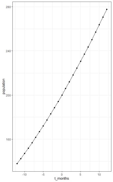
- We see that:
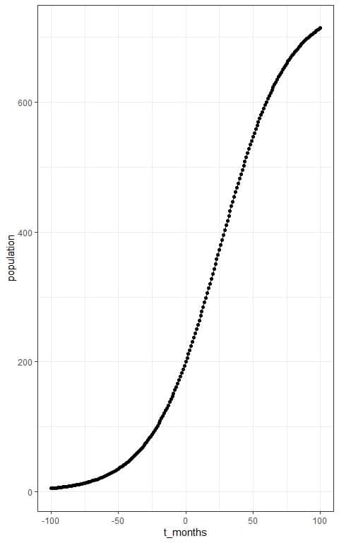
The expected number of rabbits after 12 months or 1 year= P(12) = 278 rabbits approximately. - It is a part of the Sigmoid curve and so not perfectly S-shaped.
We can see the full sigmoid curve if we extend the time boundaries to between -100 and 100.
– Application of logistic function in statistics
The logistic function can be used in logistic regression.
Logistic regression is used to model the probability of a dependent variable with two possible values, such as pass/fail given a set of one or more independent variables (predictors).
If we assume that the first level value is “fail” and the second level value is “pass” of the dependent variable.
The probability of the second level value (“pass”), p(Y = “pass”) can vary between 0 (we are certain it is a “fail” event) and 1 (certainly a “pass” event).
The formula of the logistic function that model the probability is:
p(Y)=1/(1+e^(-(β_0+β_1 x)) )
Where:
p(Y) is the probability of the second level value.
x is the independent variable value.
The quantity β_0+β_1 x is the log(odds).
We estimate the values of β_0 and β_1 such that plugging these estimates into the model for p(Y) yields a probability close to 1 for all data that have the second level value (“pass”) and a probability close to 0 for all other data that have the first level value (“fail”).
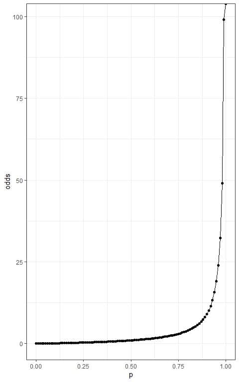
The odds of an event is the probability of an event occurring divided by the probability of not occurring.
odds = p/(1-p).
While the probability of an event can range between 0 and 1, the odds of an event can range between 0 and +∞.
When p = 0, odds = 0.
when p = 0.25, odds = 0.25/0.75 = 0.33.
when p = 0.5, odds = 0.5/0.5 = 1.
when p = 0.75, odds = 0.75*0.25 = 3.
when p = 0.95, odds = 0.95/0.05 = 19.
when p = 0.99, odds = 0.99/0.01 = 99.
when p = 1, odds = 1/0 = +∞.
The following plot plots the different probabilities on the x-axis and the resulting odds on the y-axis.
If we plot the log(odds) on the y-axis, the log(odds) have a range from -∞ to +∞.
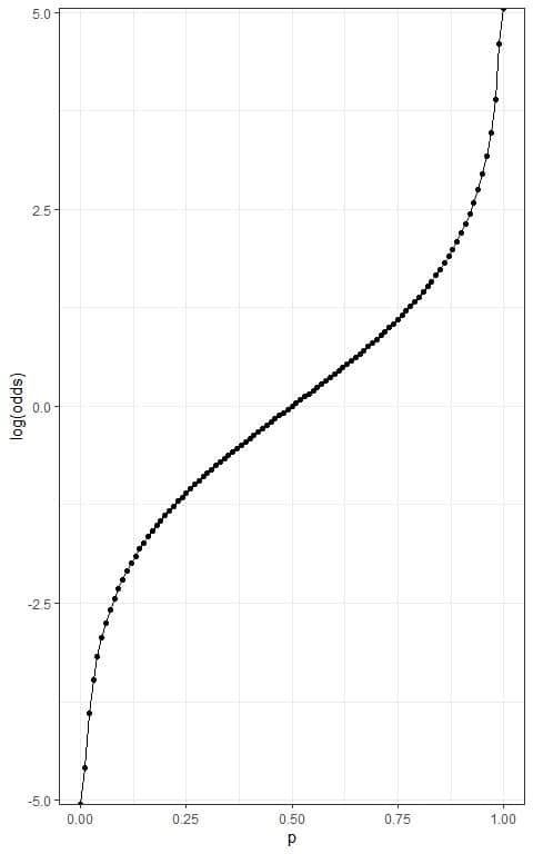
Because the log(odds) range from -∞ to +∞, they can now be put in the linear equation for a single predictor (x):
log(odds) = β_0+β_1 x
where:
β_0 is the baseline log(odds) when the predictor(x) is zero.
β_1 is the amount of log(odds) increase for each one-unit increase in x.
If β_1 is positive then increasing x will be associated with increasing the log(odds) or p(Y), and if β_1 is negative then increasing x will be associated with decreasing the log(odds) or p(Y).
For different n predictors,x_1,x_2,…..x_n:
log(odds) = β_0+β_1 x+β_2 x_2+…….+β_n x_n
and the logistic equation:
p(Y)=1/(1+e^(-(β_0+β_1 x+β_2 x_2+…….+β_n x_n)) )
p(Y)=1/(1+e^(-(log(odds))) )
p(Y)=odds/(1+odds)
– Example 1 for one predictor
The following table shows the data of 25 students illustrating the number of hours per week each student spent watching TV (tv column) and whether they passed or failed a certain exam (pass column).
The pass column has 2 values: 1 for passing and 0 for failure.
student | tv | pass |
| 1 | 0 | 1 |
2 | 0 | 1 |
| 3 | 0 | 0 |
4 | 5 | 1 |
| 5 | 7 | 1 |
| 6 | 10 | 1 |
7 | 11 | 1 |
| 8 | 12 | 1 |
9 | 14 | 1 |
| 10 | 15 | 0 |
11 | 15 | 0 |
12 | 16 | 1 |
| 13 | 17 | 0 |
14 | 19 | 0 |
| 15 | 20 | 1 |
16 | 20 | 0 |
17 | 20 | 0 |
| 18 | 23 | 0 |
19 | 24 | 0 |
20 | 25 | 0 |
| 21 | 27 | 0 |
22 | 28 | 0 |
23 | 30 | 0 |
| 24 | 30 | 0 |
25 | 32 | 1 |
We can see the relation between TV hours and pass in the following plot:
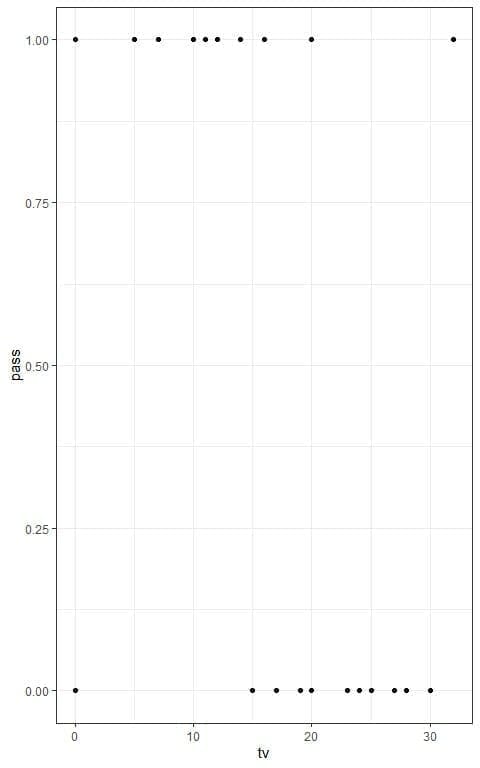
We see that increasing the number of hours watching TV is associated with more failures or less passing.
We estimate a logistic regression model for this data, assuming that pass or 1 is the second level value, and found that:
β_0 = 1.90717
β_1 for TV hours (predictor) = -0.13078.
Calculate the probability of passing for all students in this data.
We will follow these steps:
1. Estimate the log(odds) of passing for each student.
log(odds) = β_0+β_1 x = 1.90717 + -0.13078 X TV hours.
The β_1 for TV hours is negative, so increasing the number of hours watching TV will be associated with decreasing the log(odds) or probability of passing.
Update the table with a column for log(odds) of passing.
student | tv | pass | log(odds) |
| 1 | 0 | 1 | 1.90717 |
2 | 0 | 1 | 1.90717 |
3 | 0 | 0 | 1.90717 |
| 4 | 5 | 1 | 1.25327 |
5 | 7 | 1 | 0.99171 |
6 | 10 | 1 | 0.59937 |
| 7 | 11 | 1 | 0.46859 |
8 | 12 | 1 | 0.33781 |
| 9 | 14 | 1 | 0.07625 |
10 | 15 | 0 | -0.05453 |
11 | 15 | 0 | -0.05453 |
12 | 16 | 1 | -0.18531 |
| 13 | 17 | 0 | -0.31609 |
14 | 19 | 0 | -0.57765 |
| 15 | 20 | 1 | -0.70843 |
16 | 20 | 0 | -0.70843 |
| 17 | 20 | 0 | -0.70843 |
18 | 23 | 0 | -1.10077 |
| 19 | 24 | 0 | -1.23155 |
20 | 25 | 0 | -1.36233 |
| 21 | 27 | 0 | -1.62389 |
22 | 28 | 0 | -1.75467 |
23 | 30 | 0 | -2.01623 |
| 24 | 30 | 0 | -2.01623 |
25 | 32 | 1 | -2.27779 |
2., Calculate the probability of passing for each student using the logistic equation:
p(Y)=1/(1+e^(-(β_0+β_1 x)) )=1/(1+e^(-(1.90717+-0.13078x)) )=1/(1+e^(-(log(odds))) )
Update the table with a column for probability of passing for each student.
student | tv | pass | log(odds) | p(pass) |
1 | 0 | 1 | 1.90717 | 0.87070088 |
| 2 | 0 | 1 | 1.90717 | 0.87070088 |
3 | 0 | 0 | 1.90717 | 0.87070088 |
| 4 | 5 | 1 | 1.25327 | 0.77786540 |
| 5 | 7 | 1 | 0.99171 | 0.72942555 |
6 | 10 | 1 | 0.59937 | 0.64551216 |
| 7 | 11 | 1 | 0.46859 | 0.61504997 |
8 | 12 | 1 | 0.33781 | 0.58365845 |
| 9 | 14 | 1 | 0.07625 | 0.51905327 |
10 | 15 | 0 | -0.05453 | 0.48637088 |
| 11 | 15 | 0 | -0.05453 | 0.48637088 |
12 | 16 | 1 | -0.18531 | 0.45380462 |
| 13 | 17 | 0 | -0.31609 | 0.42162894 |
14 | 19 | 0 | -0.57765 | 0.35947351 |
| 15 | 20 | 1 | -0.70843 | 0.32994585 |
| 16 | 20 | 0 | -0.70843 | 0.32994585 |
17 | 20 | 0 | -0.70843 | 0.32994585 |
| 18 | 23 | 0 | -1.10077 | 0.24959565 |
19 | 24 | 0 | -1.23155 | 0.22591025 |
| 20 | 25 | 0 | -1.36233 | 0.20386188 |
21 | 27 | 0 | -1.62389 | 0.16466909 |
| 22 | 28 | 0 | -1.75467 | 0.14745914 |
23 | 30 | 0 | -2.01623 | 0.11750938 |
| 24 | 30 | 0 | -2.01623 | 0.11750938 |
25 | 32 | 1 | -2.27779 | 0.09297916 |
We see that increasing the number of TV hours is associated with decreased probability of passing this exam.
We can plot the tv hours on the x-axis and the probability on the y-axis to see the sigmoid curve of the logistic equation.
The passing and failing students are plotted as black points.
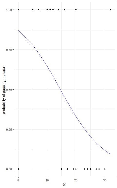
We see that the probability of passing the exam decreases with increasing the number of TV hours.
– Example 2 for two predictor
The following table shows the data of 100 persons from a certain survey.
The table shows the age of each person (age, in years), body mass index (bmi), and whether they had hypertension (hypertension, No or Yes).
age | bmi | hypertension |
| 67 | 29.02 | Yes |
63 | 33.86 | Yes |
75 | 34.03 | Yes |
| 59 | 27.73 | Yes |
68 | 28.60 | Yes |
| 70 | 29.27 | Yes |
76 | 30.08 | Yes |
| 74 | 27.46 | No |
69 | 34.31 | Yes |
| 70 | 36.10 | Yes |
68 | 24.13 | No |
| 67 | 31.44 | Yes |
62 | 34.25 | Yes |
72 | 25.22 | Yes |
| 77 | 30.08 | Yes |
63 | 25.38 | Yes |
| 78 | 29.90 | Yes |
58 | 35.78 | Yes |
| 68 | 39.51 | Yes |
67 | 29.90 | Yes |
| 65 | 29.93 | Yes |
65 | 34.47 | Yes |
| 70 | 27.26 | No |
65 | 34.41 | Yes |
| 77 | 28.89 | No |
60 | 33.62 | Yes |
| 62 | 33.24 | Yes |
62 | 28.17 | Yes |
| 63 | 31.67 | Yes |
68 | 23.57 | Yes |
| 55 | 29.49 | Yes |
74 | 31.16 | Yes |
| 56 | 30.80 | Yes |
67 | 29.41 | Yes |
| 65 | 30.13 | Yes |
60 | 27.77 | Yes |
| 55 | 32.10 | Yes |
68 | 29.03 | Yes |
| 77 | 25.47 | No |
67 | 29.48 | Yes |
| 66 | 25.39 | Yes |
72 | 23.23 | Yes |
| 61 | 33.99 | No |
58 | 29.83 | Yes |
| 75 | 25.19 | Yes |
57 | 31.64 | Yes |
| 65 | 27.81 | Yes |
70 | 24.07 | Yes |
| 68 | 30.32 | Yes |
55 | 26.40 | Yes |
| 62 | 34.45 | Yes |
77 | 34.62 | Yes |
| 56 | 30.07 | Yes |
69 | 27.29 | Yes |
| 59 | 27.30 | No |
68 | 30.00 | Yes |
61 | 29.08 | No |
| 61 | 29.86 | Yes |
70 | 33.87 | Yes |
| 75 | 31.74 | Yes |
71 | 32.38 | Yes |
| 77 | 24.03 | Yes |
65 | 28.83 | Yes |
| 76 | 37.04 | Yes |
75 | 24.18 | Yes |
| 67 | 28.73 | Yes |
59 | 33.76 | Yes |
65 | 37.04 | Yes |
| 64 | 32.59 | Yes |
71 | 27.01 | Yes |
| 57 | 27.73 | No |
62 | 32.79 | No |
68 | 27.06 | Yes |
| 76 | 39.95 | Yes |
61 | 28.35 | Yes |
67 | 29.47 | Yes |
| 55 | 23.60 | No |
64 | 39.97 | Yes |
| 72 | 30.36 | Yes |
60 | 27.79 | Yes |
65 | 27.94 | Yes |
| 66 | 27.81 | Yes |
69 | 25.61 | Yes |
| 66 | 30.67 | Yes |
68 | 26.40 | Yes |
| 65 | 30.52 | No |
60 | 33.51 | Yes |
| 76 | 27.20 | Yes |
57 | 30.85 | Yes |
| 69 | 27.12 | Yes |
67 | 34.65 | No |
62 | 25.72 | Yes |
| 72 | 28.15 | Yes |
70 | 26.90 | Yes |
| 58 | 25.78 | Yes |
68 | 31.48 | No |
| 61 | 42.53 | Yes |
76 | 31.45 | Yes |
| 64 | 25.27 | Yes |
59 | 34.19 | Yes |
We can see the relation between age and hypertension in the following box plot:
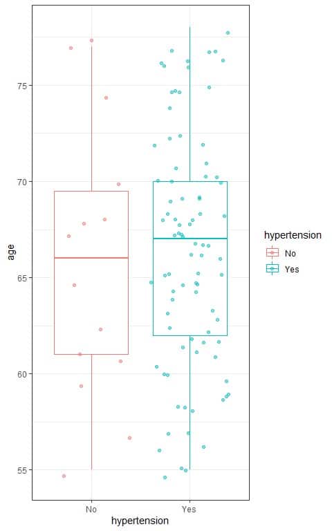
- We see that:
Persons with hypertension are plotted as blue dots while the normotensive persons are plotted as red dots. - The median age for hypertensive persons (central line of the blue box) is higher than the median age for the normotensive persons (central line of the red box).
- This may indicate that increasing age is associated with an increased probability of hypertension.
We can also see the relation between bmi and hypertension in the following box plot:
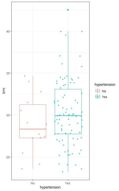
- We see that:
The median bmi for hypertensive persons (central line of the blue box) is higher than the median bmi for the normotensive persons (central line of the red box). - This may indicate that increasing body mass index is associated with increased hypertension probability.
We estimate a logistic regression model for this data, assuming that “Yes” is the second level value, and found that:
β_0 = -2.74974.
β_1 for age (predictor1) = 0.02155.
β_2 for bmi (predictor2) = 0.10631.
We will calculate the probability of developing hypertension for each person in this data by following these steps:
1. Estimate the log(odds) of hypertension for each person.
log(odds) = β_0+β_1 x_1+β_2 x_2 = -2.74974 + (0.02155 X age) + (0.10631 X bmi).
The β_1 for age is positive, so increasing age will be associated with increasing the log(odds) or the probability of hypertension.
The β_2 for bmi is positive also, so increasing the body mass index will be associated with increasing the log(odds) or the probability of hypertension.
Update the table with a column for log(odds) of hypertension.
age | bmi | hypertension | log(odds) |
| 67 | 29.02 | Yes | 1.779226 |
63 | 33.86 | Yes | 2.207567 |
| 75 | 34.03 | Yes | 2.484239 |
| 59 | 27.73 | Yes | 1.469686 |
| 68 | 28.60 | Yes | 1.756126 |
| 70 | 29.27 | Yes | 1.870454 |
| 76 | 30.08 | Yes | 2.085865 |
| 74 | 27.46 | No | 1.764233 |
| 69 | 34.31 | Yes | 2.384706 |
| 70 | 36.10 | Yes | 2.596551 |
| 68 | 24.13 | No | 1.280920 |
| 67 | 31.44 | Yes | 2.036496 |
| 62 | 34.25 | Yes | 2.227477 |
| 72 | 25.22 | Yes | 1.482998 |
| 77 | 30.08 | Yes | 2.107415 |
| 63 | 25.38 | Yes | 1.306058 |
| 78 | 29.90 | Yes | 2.109829 |
| 58 | 35.78 | Yes | 2.303932 |
| 68 | 39.51 | Yes | 2.915968 |
| 67 | 29.90 | Yes | 1.872779 |
| 65 | 29.93 | Yes | 1.832868 |
| 65 | 34.47 | Yes | 2.315516 |
| 70 | 27.26 | No | 1.656771 |
| 65 | 34.41 | Yes | 2.309137 |
| 77 | 28.89 | No | 1.980906 |
| 60 | 33.62 | Yes | 2.117402 |
| 62 | 33.24 | Yes | 2.120104 |
| 62 | 28.17 | Yes | 1.581113 |
| 63 | 31.67 | Yes | 1.974748 |
| 68 | 23.57 | Yes | 1.221387 |
| 55 | 29.49 | Yes | 1.570592 |
| 74 | 31.16 | Yes | 2.157580 |
| 56 | 30.80 | Yes | 1.731408 |
| 67 | 29.41 | Yes | 1.820687 |
| 65 | 30.13 | Yes | 1.854130 |
| 60 | 27.77 | Yes | 1.495489 |
| 55 | 32.10 | Yes | 1.848061 |
| 68 | 29.03 | Yes | 1.801839 |
| 77 | 25.47 | No | 1.617326 |
| 67 | 29.48 | Yes | 1.828129 |
| 66 | 25.39 | Yes | 1.371771 |
| 72 | 23.23 | Yes | 1.271441 |
| 61 | 33.99 | No | 2.178287 |
| 58 | 29.83 | Yes | 1.671387 |
| 75 | 25.19 | Yes | 1.544459 |
| 57 | 31.64 | Yes | 1.842258 |
| 65 | 27.81 | Yes | 1.607491 |
| 70 | 24.07 | Yes | 1.317642 |
| 68 | 30.32 | Yes | 1.938979 |
| 55 | 26.40 | Yes | 1.242094 |
| 62 | 34.45 | Yes | 2.248740 |
| 77 | 34.62 | Yes | 2.590062 |
| 56 | 30.07 | Yes | 1.653802 |
| 69 | 27.29 | Yes | 1.638410 |
| 59 | 27.30 | No | 1.423973 |
| 68 | 30.00 | Yes | 1.904960 |
| 61 | 29.08 | No | 1.656305 |
| 61 | 29.86 | Yes | 1.739227 |
| 70 | 33.87 | Yes | 2.359480 |
| 75 | 31.74 | Yes | 2.240789 |
| 71 | 32.38 | Yes | 2.222628 |
| 77 | 24.03 | Yes | 1.464239 |
| 65 | 28.83 | Yes | 1.715927 |
| 76 | 37.04 | Yes | 2.825782 |
| 75 | 24.18 | Yes | 1.437086 |
| 67 | 28.73 | Yes | 1.748396 |
| 59 | 33.76 | Yes | 2.110736 |
| 65 | 37.04 | Yes | 2.588732 |
| 64 | 32.59 | Yes | 2.094103 |
| 71 | 27.01 | Yes | 1.651743 |
| 57 | 27.73 | No | 1.426586 |
| 62 | 32.79 | No | 2.072265 |
| 68 | 27.06 | Yes | 1.592409 |
| 76 | 39.95 | Yes | 3.135145 |
| 61 | 28.35 | Yes | 1.578699 |
| 67 | 29.47 | Yes | 1.827066 |
| 55 | 23.60 | No | 0.944426 |
| 64 | 39.97 | Yes | 2.878671 |
| 72 | 30.36 | Yes | 2.029432 |
| 60 | 27.79 | Yes | 1.497615 |
| 65 | 27.94 | Yes | 1.621311 |
| 66 | 27.81 | Yes | 1.629041 |
| 69 | 25.61 | Yes | 1.459809 |
| 66 | 30.67 | Yes | 1.933088 |
| 68 | 26.40 | Yes | 1.522244 |
| 65 | 30.52 | No | 1.895591 |
| 60 | 33.51 | Yes | 2.105708 |
| 76 | 27.20 | Yes | 1.779692 |
| 57 | 30.85 | Yes | 1.758274 |
| 69 | 27.12 | Yes | 1.620337 |
| 67 | 34.65 | No | 2.377751 |
| 62 | 25.72 | Yes | 1.320653 |
| 72 | 28.15 | Yes | 1.794487 |
| 70 | 26.90 | Yes | 1.618499 |
| 58 | 25.78 | Yes | 1.240832 |
| 68 | 31.48 | No | 2.062299 |
| 61 | 42.53 | Yes | 3.086174 |
| 76 | 31.45 | Yes | 2.231510 |
| 64 | 25.27 | Yes | 1.315914 |
| 59 | 34.19 | Yes | 2.156449 |
For example, the first person has an age of 67 years and 29.02 bmi so:
log(odds) = -2.74974 + (0.02155 X67) + (0.10631X 29.02) = 1.779226.
2. Calculate the probability of hypertension for each person using the logistic equation:
p(Y)=1/(1+e^(-(β_0+β_1 x_1+β_2 x_2)) )=1/(1+e^(-(-2.74974+(0.02155Xage)+(0.10631Xbmi))) )=1/(1+e^(-(log(odds))) )
Update the table with a column for the probability of hypertension for each person.
age | bmi | hypertension | log(odds) | p(hypertension) |
67 | 29.02 | Yes | 1.779226 | 0.8556013 |
63 | 33.86 | Yes | 2.207567 | 0.9009269 |
75 | 34.03 | Yes | 2.484239 | 0.9230295 |
59 | 27.73 | Yes | 1.469686 | 0.8130097 |
68 | 28.60 | Yes | 1.756126 | 0.8527238 |
70 | 29.27 | Yes | 1.870454 | 0.8665108 |
76 | 30.08 | Yes | 2.085865 | 0.8895217 |
74 | 27.46 | No | 1.764233 | 0.8537390 |
69 | 34.31 | Yes | 2.384706 | 0.9156536 |
70 | 36.10 | Yes | 2.596551 | 0.9306393 |
68 | 24.13 | No | 1.280920 | 0.7826064 |
67 | 31.44 | Yes | 2.036496 | 0.8845760 |
62 | 34.25 | Yes | 2.227477 | 0.9026900 |
72 | 25.22 | Yes | 1.482998 | 0.8150250 |
77 | 30.08 | Yes | 2.107415 | 0.8916218 |
63 | 25.38 | Yes | 1.306058 | 0.7868527 |
78 | 29.90 | Yes | 2.109829 | 0.8918548 |
58 | 35.78 | Yes | 2.303932 | 0.9092021 |
68 | 39.51 | Yes | 2.915968 | 0.9486302 |
67 | 29.90 | Yes | 1.872779 | 0.8667795 |
65 | 29.93 | Yes | 1.832868 | 0.8621031 |
65 | 34.47 | Yes | 2.315516 | 0.9101539 |
70 | 27.26 | No | 1.656771 | 0.8398040 |
65 | 34.41 | Yes | 2.309137 | 0.9096309 |
77 | 28.89 | No | 1.980906 | 0.8787777 |
60 | 33.62 | Yes | 2.117402 | 0.8925831 |
62 | 33.24 | Yes | 2.120104 | 0.8928419 |
62 | 28.17 | Yes | 1.581113 | 0.8293620 |
63 | 31.67 | Yes | 1.974748 | 0.8781201 |
68 | 23.57 | Yes | 1.221387 | 0.7723075 |
55 | 29.49 | Yes | 1.570592 | 0.8278680 |
74 | 31.16 | Yes | 2.157580 | 0.8963749 |
56 | 30.80 | Yes | 1.731408 | 0.8495924 |
67 | 29.41 | Yes | 1.820687 | 0.8606486 |
65 | 30.13 | Yes | 1.854130 | 0.8646113 |
60 | 27.77 | Yes | 1.495489 | 0.8169007 |
55 | 32.10 | Yes | 1.848061 | 0.8638993 |
68 | 29.03 | Yes | 1.801839 | 0.8583727 |
77 | 25.47 | No | 1.617326 | 0.8344260 |
67 | 29.48 | Yes | 1.828129 | 0.8615387 |
66 | 25.39 | Yes | 1.371771 | 0.7976661 |
72 | 23.23 | Yes | 1.271441 | 0.7809894 |
61 | 33.99 | No | 2.178287 | 0.8982827 |
58 | 29.83 | Yes | 1.671387 | 0.8417607 |
75 | 25.19 | Yes | 1.544459 | 0.8241120 |
57 | 31.64 | Yes | 1.842258 | 0.8632156 |
65 | 27.81 | Yes | 1.607491 | 0.8330628 |
70 | 24.07 | Yes | 1.317642 | 0.7887891 |
68 | 30.32 | Yes | 1.938979 | 0.8742400 |
55 | 26.40 | Yes | 1.242094 | 0.7759283 |
62 | 34.45 | Yes | 2.248740 | 0.9045418 |
77 | 34.62 | Yes | 2.590062 | 0.9302193 |
56 | 30.07 | Yes | 1.653802 | 0.8394042 |
69 | 27.29 | Yes | 1.638410 | 0.8373185 |
59 | 27.30 | No | 1.423973 | 0.8059605 |
68 | 30.00 | Yes | 1.904960 | 0.8704519 |
61 | 29.08 | No | 1.656305 | 0.8397413 |
61 | 29.86 | Yes | 1.739227 | 0.8505888 |
70 | 33.87 | Yes | 2.359480 | 0.9136848 |
75 | 31.74 | Yes | 2.240789 | 0.9038531 |
71 | 32.38 | Yes | 2.222628 | 0.9022632 |
77 | 24.03 | Yes | 1.464239 | 0.8121802 |
65 | 28.83 | Yes | 1.715927 | 0.8476035 |
76 | 37.04 | Yes | 2.825782 | 0.9440533 |
75 | 24.18 | Yes | 1.437086 | 0.8080030 |
67 | 28.73 | Yes | 1.748396 | 0.8517504 |
59 | 33.76 | Yes | 2.110736 | 0.8919423 |
65 | 37.04 | Yes | 2.588732 | 0.9301329 |
64 | 32.59 | Yes | 2.094103 | 0.8903287 |
71 | 27.01 | Yes | 1.651743 | 0.8391265 |
57 | 27.73 | No | 1.426586 | 0.8063689 |
62 | 32.79 | No | 2.072265 | 0.8881781 |
68 | 27.06 | Yes | 1.592409 | 0.8309547 |
76 | 39.95 | Yes | 3.135145 | 0.9583194 |
61 | 28.35 | Yes | 1.578699 | 0.8290201 |
67 | 29.47 | Yes | 1.827066 | 0.8614118 |
55 | 23.60 | No | 0.944426 | 0.7199928 |
64 | 39.97 | Yes | 2.878671 | 0.9467819 |
72 | 30.36 | Yes | 2.029432 | 0.8838527 |
60 | 27.79 | Yes | 1.497615 | 0.8172185 |
65 | 27.94 | Yes | 1.621311 | 0.8349759 |
66 | 27.81 | Yes | 1.629041 | 0.8360382 |
69 | 25.61 | Yes | 1.459809 | 0.8115035 |
66 | 30.67 | Yes | 1.933088 | 0.8735908 |
68 | 26.40 | Yes | 1.522244 | 0.8208687 |
65 | 30.52 | No | 1.895591 | 0.8693917 |
60 | 33.51 | Yes | 2.105708 | 0.8914567 |
76 | 27.20 | Yes | 1.779692 | 0.8556588 |
57 | 30.85 | Yes | 1.758274 | 0.8529933 |
69 | 27.12 | Yes | 1.620337 | 0.8348416 |
67 | 34.65 | No | 2.377751 | 0.9151149 |
62 | 25.72 | Yes | 1.320653 | 0.7892904 |
72 | 28.15 | Yes | 1.794487 | 0.8574765 |
70 | 26.90 | Yes | 1.618499 | 0.8345880 |
58 | 25.78 | Yes | 1.240832 | 0.7757088 |
68 | 31.48 | No | 2.062299 | 0.8871845 |
61 | 42.53 | Yes | 3.086174 | 0.9563188 |
76 | 31.45 | Yes | 2.231510 | 0.9030436 |
64 | 25.27 | Yes | 1.315914 | 0.7885010 |
59 | 34.19 | Yes | 2.156449 | 0.8962699 |
If we plot the age on the x-axis and the hypertension probability on the y-axis, we will not see the sigmoid curve of the logistic equation.
We see a zipped curve because our logistic equation also takes account of the bmi.
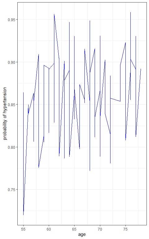
We can plot the bmi on the x-axis and the probability on the y-axis with a separate line for each age to see the sigmoid curve of the logistic equation.
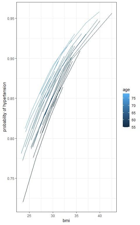
We see that increasing age (light blue lines) or bmi is associated with an increased probability of hypertension.
4. Practice questions
1. A population of tigers in a certain forest has a growth rate of 0.06 or 6% per year, with a carrying capacity of 136 tigers.
If the initial population was 30 tigers, draw the logistic curve of growth for this population.
2. In the above example, if the initial population was 200 tigers, draw the logistic curve of growth for this population.
3. From certain data, we estimate a logistic regression model for the effect of age on developing cardiovascular (cv) events, assuming that the presence of cv is the second level value, and found that:
β_0 = -4.426704.
β_1 for age (predictor) = 0.023421.
Calculate the probability of developing cv events for the age range 20-80 years.
4. From certain data, we estimate a logistic regression model for the effect of age on developing Type-2 diabetes (diab), assuming that the presence of Type-2 diabetes is the second level value, and found that:
β_0 = -1.67193.
β_1 for age (predictor) = 0.02343.
Calculate the probability of developing Type-2 diabetes for the age range 20-80 years.
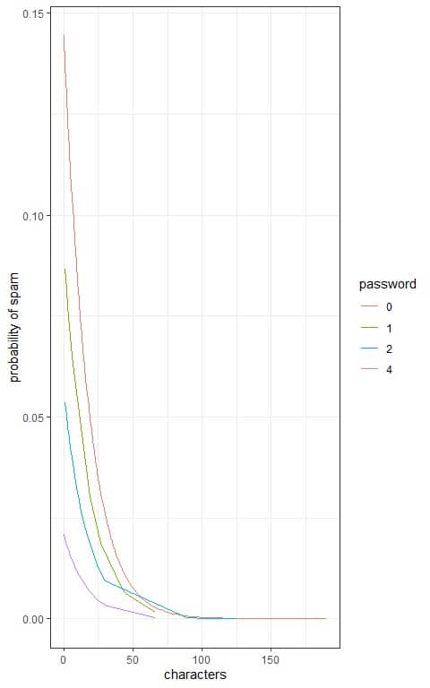
5. The following plot shows the logistic regression curves that determine the effect of the number of characters in the email, in thousands, and the number of times “password” appeared in the email on the probability of spam email.
How do these 2 predictors affect the probability of an email being spam?
5. Answer key
1. The growth rate is per year so the x-axis will be in years.
We know that the population at the current year or t = 0 is 30. We use the logistic equation to know the population size for any year:
P(t)=K/(1+((K-P_0)/P_0 )e^(-rt) )=136/(1+((136-30)/30)e^(-0.06t) )
For example, at time = 0:
The population size at time = 0 = P(0) = 136/1+(136-30/30)Xe^(-0.06X0) = 136/(1+((136-30)/30))= 30.
Using the above formula, we can calculate the population size for the past and next 20 years and produce that table.
year | population |
-20 | 10.68252 |
-19 | 11.28826 |
-18 | 11.92508 |
-17 | 12.59420 |
-16 | 13.29684 |
-15 | 14.03422 |
-14 | 14.80756 |
-13 | 15.61806 |
-12 | 16.46689 |
-11 | 17.35520 |
-10 | 18.28411 |
-9 | 19.25466 |
-8 | 20.26787 |
-7 | 21.32464 |
-6 | 22.42585 |
-5 | 23.57223 |
-4 | 24.76443 |
-3 | 26.00299 |
-2 | 27.28829 |
-1 | 28.62060 |
0 | 30.00000 |
1 | 31.42643 |
2 | 32.89963 |
3 | 34.41916 |
4 | 35.98437 |
5 | 37.59442 |
6 | 39.24825 |
7 | 40.94455 |
8 | 42.68182 |
9 | 44.45834 |
10 | 46.27213 |
11 | 48.12102 |
12 | 50.00261 |
13 | 51.91432 |
14 | 53.85334 |
15 | 55.81671 |
16 | 57.80130 |
17 | 59.80382 |
18 | 61.82087 |
19 | 63.84895 |
20 | 65.88446 |
Plot the year values on the x-axis and the population size on the y-axis.
Connect the intersecting points with a line to draw the sigmoid curve.
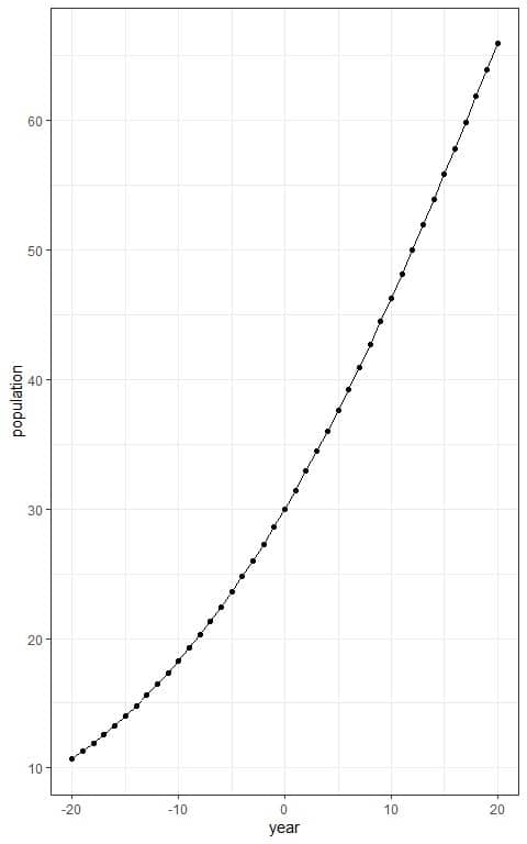
For example, the expected number of tigers after 20 years= P(20) = 66 tigers approximately.
2. The initial population is larger than the carrying capacity so the population will decrease with years.
We know that the population at the current year or t = 0 is 200. We use the logistic equation to know the population size for any year:
P(t)=K/(1+((K-P_0)/P_0 )e^(-rt) )=136/(1+((136-200)/200)e^(-0.06t) )
For example, at time = 0:
The population size at time = 0 = P(0) = 136/1+(136-200/200)Xe^(-0.06X0) = 136/(1+((136-200)/200))= 200.
Using the above formula, we can calculate the population size for the past and next 10 years and produce that table.
year | population |
-10 | 326.2001 |
-9 | 301.6338 |
-8 | 281.6574 |
-7 | 265.1215 |
-6 | 251.2309 |
-5 | 239.4176 |
-4 | 229.2649 |
-3 | 220.4605 |
-2 | 212.7656 |
-1 | 205.9943 |
0 | 200.0000 |
1 | 194.6652 |
2 | 189.8949 |
3 | 185.6114 |
4 | 181.7504 |
5 | 178.2582 |
6 | 175.0900 |
7 | 172.2075 |
8 | 169.5783 |
9 | 167.1746 |
10 | 164.9724 |
Plot the year values on the x-axis and the population size on the y-axis.
Connect the intersecting points with a line to draw the sigmoid curve.
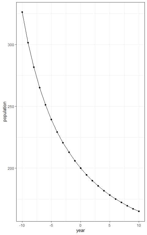
For example, the expected number of tigers after 10 years= P(10) = 165 tigers approximately.
3. Estimate the log(odds) of developing cv event for each age value.
log(odds) = β_0+β_1 x = -4.426704 + 0.023421 X age.
The β_1 for age is positive, so increasing age will be associated with increasing the log(odds) or probability of cv event.
The following table will be produced.
age | log(odds) |
20 | -3.958284 |
21 | -3.934863 |
22 | -3.911442 |
23 | -3.888021 |
24 | -3.864600 |
25 | -3.841179 |
26 | -3.817758 |
27 | -3.794337 |
28 | -3.770916 |
29 | -3.747495 |
30 | -3.724074 |
31 | -3.700653 |
32 | -3.677232 |
33 | -3.653811 |
34 | -3.630390 |
35 | -3.606969 |
36 | -3.583548 |
37 | -3.560127 |
38 | -3.536706 |
39 | -3.513285 |
40 | -3.489864 |
41 | -3.466443 |
42 | -3.443022 |
43 | -3.419601 |
44 | -3.396180 |
45 | -3.372759 |
46 | -3.349338 |
47 | -3.325917 |
48 | -3.302496 |
49 | -3.279075 |
50 | -3.255654 |
51 | -3.232233 |
52 | -3.208812 |
53 | -3.185391 |
54 | -3.161970 |
55 | -3.138549 |
56 | -3.115128 |
57 | -3.091707 |
58 | -3.068286 |
59 | -3.044865 |
60 | -3.021444 |
61 | -2.998023 |
62 | -2.974602 |
63 | -2.951181 |
64 | -2.927760 |
65 | -2.904339 |
66 | -2.880918 |
67 | -2.857497 |
68 | -2.834076 |
69 | -2.810655 |
70 | -2.787234 |
71 | -2.763813 |
72 | -2.740392 |
73 | -2.716971 |
74 | -2.693550 |
75 | -2.670129 |
76 | -2.646708 |
77 | -2.623287 |
78 | -2.599866 |
79 | -2.576445 |
80 | -2.553024 |
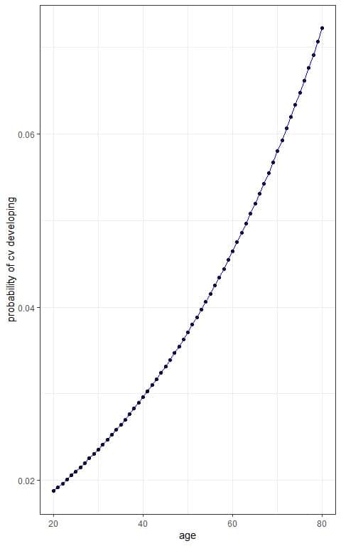
Calculate the probability of cv developing for each age using the logistic equation:
p(Y)=1/(1+e^(-(β_0+β_1 x) )=1/(1+e^(-(-4.426704+0.023421x)) )=1/(1+e^(-(log(odds))) )
Update the table with a column for probability of cv developing for each age value.
age | log(odds) | p(cv) |
20 | -3.958284 | 0.01873804 |
21 | -3.934863 | 0.01917357 |
22 | -3.911442 | 0.01961902 |
23 | -3.888021 | 0.02007460 |
24 | -3.864600 | 0.02054055 |
25 | -3.841179 | 0.02101707 |
26 | -3.817758 | 0.02150442 |
27 | -3.794337 | 0.02200280 |
28 | -3.770916 | 0.02251247 |
29 | -3.747495 | 0.02303367 |
30 | -3.724074 | 0.02356665 |
31 | -3.700653 | 0.02411165 |
32 | -3.677232 | 0.02466894 |
33 | -3.653811 | 0.02523878 |
34 | -3.630390 | 0.02582143 |
35 | -3.606969 | 0.02641716 |
36 | -3.583548 | 0.02702626 |
37 | -3.560127 | 0.02764901 |
38 | -3.536706 | 0.02828569 |
39 | -3.513285 | 0.02893659 |
40 | -3.489864 | 0.02960201 |
41 | -3.466443 | 0.03028226 |
42 | -3.443022 | 0.03097764 |
43 | -3.419601 | 0.03168847 |
44 | -3.396180 | 0.03241506 |
45 | -3.372759 | 0.03315775 |
46 | -3.349338 | 0.03391685 |
47 | -3.325917 | 0.03469271 |
48 | -3.302496 | 0.03548566 |
49 | -3.279075 | 0.03629606 |
50 | -3.255654 | 0.03712425 |
51 | -3.232233 | 0.03797059 |
52 | -3.208812 | 0.03883545 |
53 | -3.185391 | 0.03971920 |
54 | -3.161970 | 0.04062221 |
55 | -3.138549 | 0.04154486 |
56 | -3.115128 | 0.04248754 |
57 | -3.091707 | 0.04345063 |
58 | -3.068286 | 0.04443455 |
59 | -3.044865 | 0.04543968 |
60 | -3.021444 | 0.04646645 |
61 | -2.998023 | 0.04751527 |
62 | -2.974602 | 0.04858655 |
63 | -2.951181 | 0.04968072 |
64 | -2.927760 | 0.05079822 |
65 | -2.904339 | 0.05193949 |
66 | -2.880918 | 0.05310496 |
67 | -2.857497 | 0.05429508 |
68 | -2.834076 | 0.05551031 |
69 | -2.810655 | 0.05675111 |
70 | -2.787234 | 0.05801794 |
71 | -2.763813 | 0.05931127 |
72 | -2.740392 | 0.06063157 |
73 | -2.716971 | 0.06197933 |
74 | -2.693550 | 0.06335503 |
75 | -2.670129 | 0.06475916 |
76 | -2.646708 | 0.06619220 |
77 | -2.623287 | 0.06765466 |
78 | -2.599866 | 0.06914704 |
79 | -2.576445 | 0.07066985 |
80 | -2.553024 | 0.07222359 |
We see that increasing age is associated with an increased probability of developing cv.
We can plot the age on the x-axis and the probability on the y-axis to see the sigmoid curve of the logistic equation.
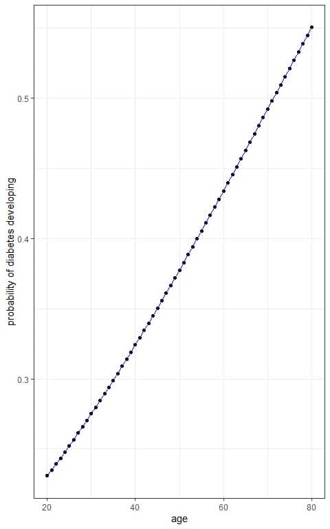
4. Estimate the log(odds) of developing Type-2 diabetes for each age value.
log(odds) = β_0+β_1 x = -1.67193 + 0.02343 X age.
The β_1 for age is positive, so increasing age will be associated with increasing the log(odds) or probability of Type-2 diabetes.
The following table will be produced.
age | log(odds) |
20 | -1.20333 |
21 | -1.17990 |
22 | -1.15647 |
23 | -1.13304 |
24 | -1.10961 |
25 | -1.08618 |
26 | -1.06275 |
27 | -1.03932 |
28 | -1.01589 |
29 | -0.99246 |
30 | -0.96903 |
31 | -0.94560 |
32 | -0.92217 |
33 | -0.89874 |
34 | -0.87531 |
35 | -0.85188 |
36 | -0.82845 |
37 | -0.80502 |
38 | -0.78159 |
39 | -0.75816 |
40 | -0.73473 |
41 | -0.71130 |
42 | -0.68787 |
43 | -0.66444 |
44 | -0.64101 |
45 | -0.61758 |
46 | -0.59415 |
47 | -0.57072 |
48 | -0.54729 |
49 | -0.52386 |
50 | -0.50043 |
51 | -0.47700 |
52 | -0.45357 |
53 | -0.43014 |
54 | -0.40671 |
55 | -0.38328 |
56 | -0.35985 |
57 | -0.33642 |
58 | -0.31299 |
59 | -0.28956 |
60 | -0.26613 |
61 | -0.24270 |
62 | -0.21927 |
63 | -0.19584 |
64 | -0.17241 |
65 | -0.14898 |
66 | -0.12555 |
67 | -0.10212 |
68 | -0.07869 |
69 | -0.05526 |
70 | -0.03183 |
71 | -0.00840 |
72 | 0.01503 |
73 | 0.03846 |
74 | 0.06189 |
75 | 0.08532 |
76 | 0.10875 |
77 | 0.13218 |
78 | 0.15561 |
79 | 0.17904 |
80 | 0.20247 |
Calculate the probability of developing Type-2 diabetes for each age value using the logistic equation:
p(Y)=1/(1+e^(-(β_0+β_1 x)) )=1/(1+e^(-(-1.67193+0.02343x)) )=1/(1+e^(-(log(odds))) )
Update the table with a column for probability of developing Type-2 diabetes for each age value.
age | log(odds) | p(diab) |
20 | -1.20333 | 0.2308834 |
21 | -1.17990 | 0.2350702 |
22 | -1.15647 | 0.2393093 |
23 | -1.13304 | 0.2436005 |
24 | -1.10961 | 0.2479436 |
25 | -1.08618 | 0.2523383 |
26 | -1.06275 | 0.2567843 |
27 | -1.03932 | 0.2612812 |
28 | -1.01589 | 0.2658288 |
29 | -0.99246 | 0.2704265 |
30 | -0.96903 | 0.2750739 |
31 | -0.94560 | 0.2797706 |
32 | -0.92217 | 0.2845159 |
33 | -0.89874 | 0.2893095 |
34 | -0.87531 | 0.2941506 |
35 | -0.85188 | 0.2990386 |
36 | -0.82845 | 0.3039729 |
37 | -0.80502 | 0.3089527 |
38 | -0.78159 | 0.3139773 |
39 | -0.75816 | 0.3190459 |
40 | -0.73473 | 0.3241576 |
41 | -0.71130 | 0.3293117 |
42 | -0.68787 | 0.3345071 |
43 | -0.66444 | 0.3397429 |
44 | -0.64101 | 0.3450183 |
45 | -0.61758 | 0.3503320 |
46 | -0.59415 | 0.3556832 |
47 | -0.57072 | 0.3610707 |
48 | -0.54729 | 0.3664934 |
49 | -0.52386 | 0.3719501 |
50 | -0.50043 | 0.3774396 |
51 | -0.47700 | 0.3829608 |
52 | -0.45357 | 0.3885123 |
53 | -0.43014 | 0.3940929 |
54 | -0.40671 | 0.3997013 |
55 | -0.38328 | 0.4053360 |
56 | -0.35985 | 0.4109959 |
57 | -0.33642 | 0.4166794 |
58 | -0.31299 | 0.4223851 |
59 | -0.28956 | 0.4281116 |
60 | -0.26613 | 0.4338574 |
61 | -0.24270 | 0.4396211 |
62 | -0.21927 | 0.4454011 |
63 | -0.19584 | 0.4511959 |
64 | -0.17241 | 0.4570040 |
65 | -0.14898 | 0.4628237 |
66 | -0.12555 | 0.4686537 |
67 | -0.10212 | 0.4744922 |
68 | -0.07869 | 0.4803376 |
69 | -0.05526 | 0.4861885 |
70 | -0.03183 | 0.4920432 |
71 | -0.00840 | 0.4979000 |
72 | 0.01503 | 0.5037574 |
73 | 0.03846 | 0.5096138 |
74 | 0.06189 | 0.5154676 |
75 | 0.08532 | 0.5213171 |
76 | 0.10875 | 0.5271607 |
77 | 0.13218 | 0.5329970 |
78 | 0.15561 | 0.5388242 |
79 | 0.17904 | 0.5446408 |
80 | 0.20247 | 0.5504453 |
We see that increasing age is associated with an increased probability of developing Type-2 diabetes.
We can plot the age on the x-axis and the probability on the y-axis to see the sigmoid curve of the logistic equation.
5. Increasing the number of characters in the email is associated with decreased probability of spam email.
Also, increasing the number of times “password” appeared in the email (from 0 to 4) is associated with decreased probability of spam email for a constant small number of characters.