Matrices – Explanation

Matrices are a rectangular arrangement of numbers in rows and columns. They are known as arrays as well. In this article, we are going to learn about matrices, what can be done with them, how to recognize and read them, and some real life examples where matrices are used. Let’s get started with the definition of matrices:

Matrices are ordered set of rectangular numbers, or expressions, arranged in rows and columns.

Let’s dive into the nitty – gritty of matrices.

What is a matrix?

As already mentioned, matrix is a rectangular arrangement of numbers in rows and columns. Matrices are the plural from of a matrix. A matrix is shown below:

\begin{bmatrix} 2 & { – 1 } \\ 6 & 5 \end {bmatrix}

The numbers, variables, or expressions inside the matrix are called the entries or elements of a matrix. This matrix shows numbers as the elements. This is a $ 2 \times 2 $ matrix. It is pronounced as a (two – by – two) matrix. This name of a matrix is known as its dimensions. Since this matrix has 2 rows and 2 columns, we name it a $ 2 \times 2 $ matrix (two-by-two matrix). You can read more about dimensions of a matrix in this article here.

How to read a matrix?

We read a matrix from left-to-right and then from top-to-bottom. We note down the number of rows when we go from left-to-right and number of columns when going top-to-bottom. This gives us the dimension of a matrix, or, its order. When naming matrices, we put the number of rows first and then the number of columns. You can read more about it here, in the article on dimensions of a matrix.

We have denoted our example matrix with brackets “[” and “]”. We can also denote the rectangular arrangement of numbers with parenthesis, such as “(” and “)”. We show the same matrix with parenthesis below:

\begin{pmatrix} 2 & { – 1 } \\ 6 & 5 \end {pmatrix}

Both of these matrices are the same. They are a $ 2 \times 2 $ matrix. We can also have matrices consisting of rows or columns, only.

A matrix with only row(s) is shown below:

\begin{bmatrix} 3 & { – 1 } & { – 1 0 }  \end {bmatrix}

This is also a matrix but with only $ 1 $ row. The dimensions of this matrix is $ 1 \times 3 $ (1 by 3 matrix). This means, it has $ 1 $ row and $ 3 $ columns.

A matrix with only column(s) is shown below:

\begin{bmatrix} { 0 } \\ { 0 } \\ { 3 } \end {bmatrix}

This is also a matrix but with only $ 1 $ column. The dimensions of this matrix is $ 3 \times 1 $ (3 by 1 matrix). This means, it has $ 3 $ rows and $ 1 $ column.

We can name a matrix with letters as well. The use of capital letters is conventional. Below we show an example of two matrices named A and B:

$ A = \begin{bmatrix} 3 & 10 \\ { 0 } & 20 \end {bmatrix} $

$ B = \begin{bmatrix} 1 & { – 8 } \\ { – 40 } & 6 \end {bmatrix} $

The first matrix can be called “Matrix A” and the second one “Matrix B”. Moreover, we can denote these two matrix with subscript notation.

The first matrix can be called as $ A_{2 , 2} $ and the second matrix can be called as $ B_{2 , 2} $. The first number in the subscript is the number of rows and the next number is the number of columns.

We can also refer each element of a matrix by the subscript notation. Note the matrix below:

$ C = \begin{bmatrix} 3 & { – 3 } \\ 4 & { – 4 } \end {bmatrix} $

When we note $ C_{ 1 2 } $, we refer to the element in Matrix $ C $ that is located on the first row and second column. Looking at Matrix $ C $,

$ C_{ 1 2 } = – 3  $

When we note $ C_{ 2 2 } $, we refer to the element in Matrix $ C $ that is located in the second row and second column. Looking at Matrix $ C $,

$ C_{ 2 2 } = – 4  $

The first number in the subscript is the row location of the element and the second number is the column location.

Using subscript notation, the difference in referring to a matrix verses referring to a single entry in a matrix  is just a comma, ‘,‘. 

Equivalent Matrices

When $ 2 $ matrices have the same number of rows and same number of columns and all their elements are same, they are called equivalent matrices.

$ \begin{bmatrix} { – 1 } & { – 2 } \\ { – 3 } & { – 4 } \end {bmatrix} =  \begin{bmatrix} { – 1 } & { – 2 } \\ { – 3 } & { – 4 } \end {bmatrix} $

The two matrices shown above are equivalent matrices because they have the same number of rows and columns ($ 2 $ rows and $ 2 $ columns) and all the $ 4 $ elements, or entries, are the same.

Moreover, this is also a square matrix. When the number of rows equals the number of columns, it is known as a square matrix.

Diagonal of a Matrix

The diagonal of a matrix goes from the upper left corner to the lower right corner, or from upper right corner to the lower left corner. We have diagonal in square matrices only.

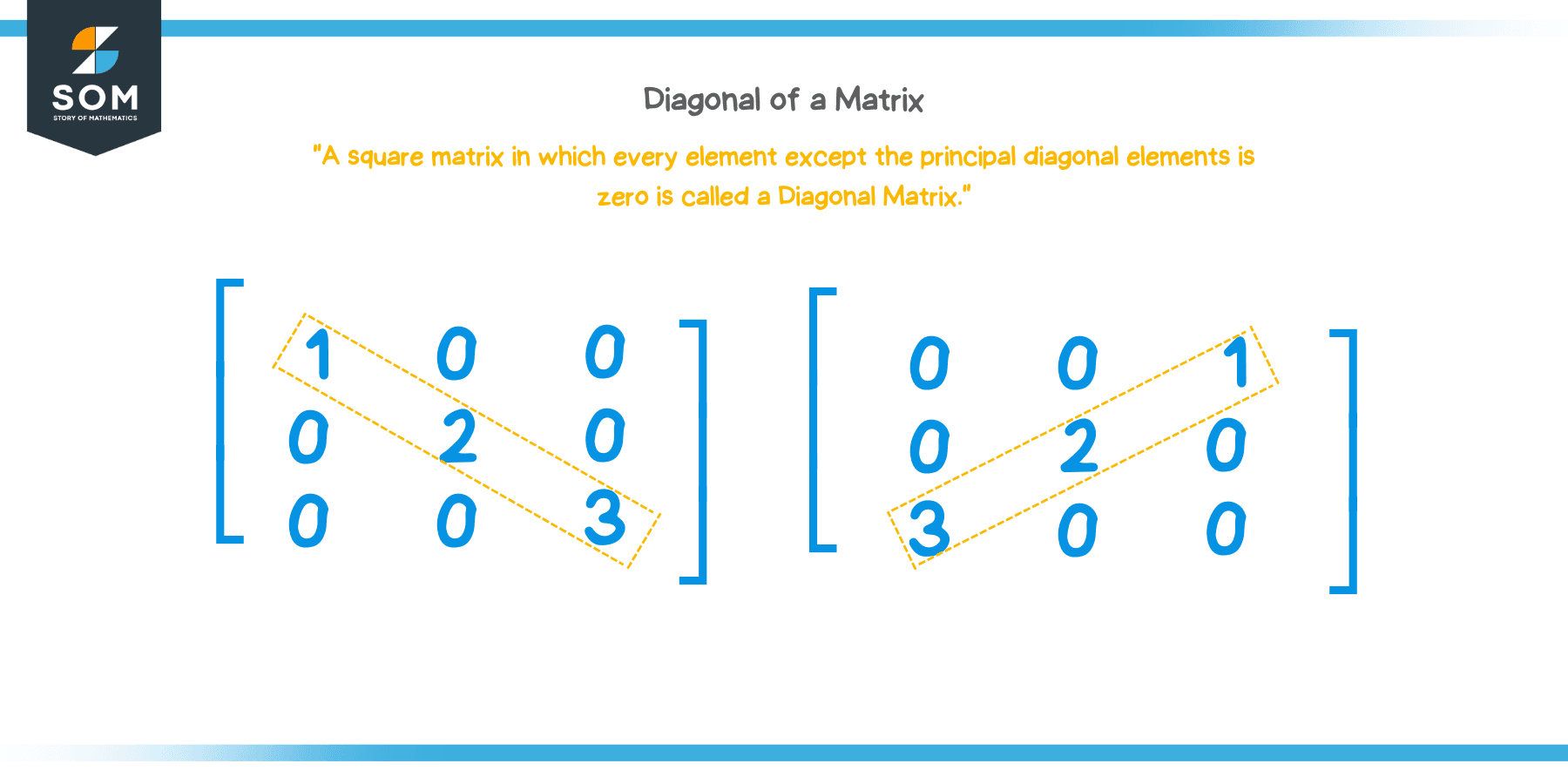The matrix shown above is a $ 3 \times 3 $ matrix. The diagonal from upper left corner to lower right corner is highlighted in red. This is also known as the principal diagonal of a matrix.

This picture above shows the diagonal from upper right corner to lower left corner (highlighted in red). This is also known as the secondary diagonal of a matrix.

When all entries in a matrix are $ { 0 } $, besides the diagonal, we call it a diagonal matrix. An example of a diagonal matrix is shown below:

\begin{bmatrix} 1 & { 0 } & { 0 } \\ { 0 } & 5 & { 0 } \\ { 0 } & { 0 } & 6 \end {bmatrix}

Please note the play with words. Diagonal matrix is a matrix where all the entries are $ 0 $ besides the diagonal and the diagonal of a matrix is just the collection of entries from corner to corner.

How to do matrices?

We can do some basic arithmetic operations on matrices, just like we do with numbers. Operations are basically procedures that we do on matrices. Just like numbers, we can add, subtract, and multiply matrices. There isn’t any such thing as matrix division. If we were to divide Matrix A by Matrix B, we would instead multiply Matrix A by the inverse of Matrix B. More on it later.

Let’s look at some briefs on the basic operations with matrices.

Matrix Addition

We can add two matrix if their orders (dimension) are the same. If two matrices have the same number of rows and columns, we can add them. We simply add the corresponding values of each matrix to each other and come up with the resultant matrix that has the same order (same number of rows and columns). Check the below example:

Matrix A and B:

$ A = \begin{bmatrix} 0 & 2 \\ 1 & 3 \end {bmatrix} $

$ B = \begin{bmatrix} { – 2 } & 3 \\ 1 & 0 \end {bmatrix} $

The addition of Matrix A and Matrix B:

$ A + B = \begin{bmatrix} { 0 + ( – 2 ) } & { 2 + 3 } \\ { 1 + 1 } & { 3 + 0 } \end {bmatrix} $

$ A + B = \begin{bmatrix} { – 2 } & 5 \\ 2 & 3 \end {bmatrix} $

Note how we added the corresponding entries in each matrix together to get the resultant matrix.

Matrix addition isn’t possible with matrices of different orders (dimensions). Next, let us look at matrix subtraction.

Matrix Subtraction

We can subtract two matrix if their orders are the same. If two matrices have the same number of rows and columns, we can subtract them. Just like matrix addition, we subtract the corresponding values of each matrix to each other and come up with the resultant matrix that has the same order (same number of rows and columns). Let’s take a look at an example of matrix subtraction:

Matrix C and D:

$ C = \begin{bmatrix} { – 1 } & { – 3 } \\ 1 & 0 \end {bmatrix} $

$ D = \begin{bmatrix} 8 & { – 1 } \\ 2 & 0 \end {bmatrix} $

The subtraction of Matrix C and Matrix D:

$ C – D = \begin{bmatrix} { { – 1 } – 8 } & { { – 3 } – ( – 1 ) } \\ { 1 – 2 } & { 0 – 0 } \end {bmatrix} $

$ C – D = \begin{bmatrix} { – 9 } & { – 2 } \\ { – 1 } & 0 \end {bmatrix} $

Note how we subtracted the corresponding entries in each matrix together to get the resultant matrix.

Just like matrix addition, matrix subtraction isn’t possible with matrices of different orders (dimensions).

Matrix Multiplication

There are $ 2 $ types of matrix multiplication, scalar multiplication and normal matrix multiplication. Scalar multiplication is when you multiply a matrix by a scalar quantity. Matrix multiplication is the process of multiplying two matrices.

In scalar multiplication, we multiply a matrix by a constant. We multiply each entry (element) by the scalar quantity. That’s it. We have the resultant matrix.

Consider the matrix shown below:

\begin{bmatrix} 3 & 2 \\ { 0 } & { – 3 } \end {bmatrix}

If we were to multiply this matrix with the quantity $ 2 $, we would simply multiply each entry by $ 2 $. The process is shown below:

$ 2 \times \begin{bmatrix} 3 & 2 \\ { 0 } & { – 3 } \end {bmatrix} $

$ =  \begin{bmatrix} 6 & 4 \\ { 0 } & { – 6 } \end {bmatrix} $

Thus, for scalar multiplication, we multiply each entry of a matrix with the scalar quantity.

In matrix multiplication where we are multiplying $ 2 $ matrices, we have to make sure the number of columns of the first matrix matches the number of rows of the second matrix. If they don’t we cannot multiply the matrices.

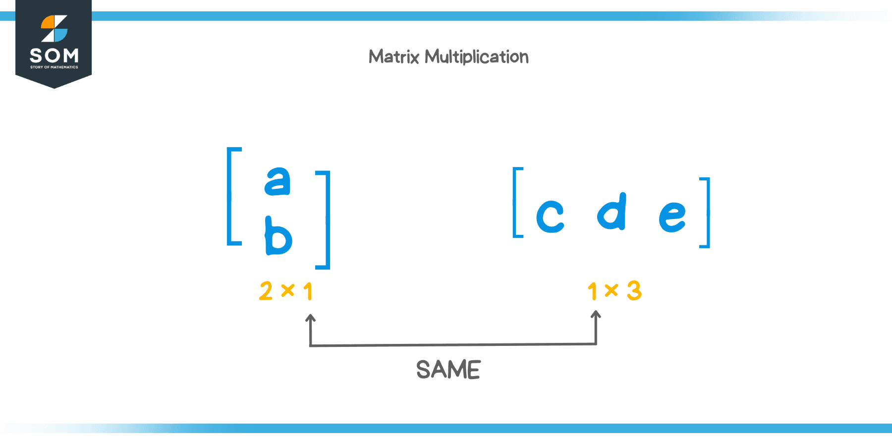The first matrix (left hand side) has $ 2 $ rows and $ 1 $ column. Hence the dimension of the matrix (written below) is $ 2 \times 1 $. The second matrix (right hand side) has $ 1 $ row and $ 3 $ column. Its dimension is $ 1 \times 3 $.

The number of column(s) is equal to the number of row(s). Hence, matrix multiplication is possible. Remember, the number of columns in the first matrix MUST equal the number of rows in the second matrix, not vice versa. The multiplication process isn’t shown in this article. But if we were to do the multiplication, the resultant matrix would have had an order of $ m \times n $, where $ m $ is the number of rows of the first matrix and $ n $ is the number of columns of the second matrix. You can read the details of matrix multiplication here.

Matrix Division

As mentioned before, matrix division isn’t possible. It is an undefined operation. We can easily add, subtract, and multiply matrices just as we do with numbers. But matrix division takes a different approach. Suppose we want to divide Matrix A by Matrix B. We would find the inverse of Matrix B and then multiply that inverse with Matrix A.

$ \frac{ A }{ B } = A \times { B } ^ { – 1 } $

$ B  ^ { – 1 } $ is the inverse matrix of $ B $. Not all matrices have inverses. First of all, it has to be a square matrix for it to have an inverse. Even then, not all square matrices have inverses. We won’t get into the details of an inverse matrix. If you want to know the particulars, please read the article on inverse matrices, here.

What are matrices used for?

Matrices are mostly used in higher field of studies. At a lower level, extracting information from word problems and arranging them into a rectangular format is the use of matrices. At high school level, information from linear equations in $ 2 $ or $ 3 $ variables are extracted and formed into a matrix. Operations on such matrices leads us to find the intersection point(s) of lines very easily. In college and beyond, you learn that matrices are the basis of linear algebra and vector calculus.

Matrices are widely used in the field of:

• Image processing
• Genetic Analysis
• Weather system models
• Digital signal processing
• Quantum mechanics

Summary

We have learned a lot of information in this lesson. Let’s do a quick summary on what we have learned.

• Matrices are a rectangular arrangement of numbers in rows and columns.
• The entries inside a matrix are known as the elements of a matrix.
• The dimension of a matrix is the number of rows and the number of column it has.
• A capital letter can be used to name  a matrix as well.
• The subscript notation of naming a matrix, for example $ A_{ 3 2 }  $ tells us that Matrix A has $ 3 $ rows and $ 2 $ columns. The first number in the subscript is the number of rows and the second number is the number of columns the matrix has.
• A square matrix is a matrix whose number of rows and columns are the same.
• Equivalent matrices are square matrices in which all the elements of each matrix are the same.
• The diagonal of a matrix are the entries going from top left corner to the bottom right corner. This is the principal diagonal. The secondary diagonal is when you take the entries from the top right to the bottom left.
• Diagonal matrix is a matrix in which all the entries, besides the primary diagonal, are $ 0 $.
• We can add, subtract, and multiply matrices. The operation of division is undefined.
• Matrix addition between two matrices are done by adding the corresponding entries in each matrix. For matrix addition to be defined, the dimensions of both matrices have to be the same.
• Matrix subtraction between two matrices are done by subtracting the corresponding entries in each matrix. For matrix subtraction to be defined, the dimensions of both matrices have to be the same.
• Matrix multiplication is of $ 2 $ types, scalar multiplication and matrix multiplication. Scalar multiplication is when we multiply a scalar quantity with a matrix. We do this by simply multiplying each entry of the matrix by the scalar. Matrix multiplication is defined and can be done if the number of column(s) of the first matrix is the same as the number of row(s) of the second matrix. The resultant matrix has an order of $ m \times n $, where $ m $ is the number of rows of the first matrix and $ n $ is the number of columns of the second matrix.
• To divide Matrix $ A $ by Matrix $ B $, we multiply Matrix $ A $ with the inverse matrix of $ B $.
• Matrices are used in a variety of fields in real life. Some of the usage of matrices are in solving linear equations in multi dimensions, digital image processing, digital signal processing, quantum mechanics etc.

Hopefully, we have a firm understanding of what matrices are, how to denote them, what operations we can perform, and their uses. Now, we can clarify our knowledge on matrices with the help of numerous examples shown below.

Example 1

Identify each of the following as a matrix or not a matrix. If it isn’t a matrix, state the reason.

1. $ \begin{bmatrix} a & b \\ c & d \end {bmatrix} $
2. 
3. $ \begin{bmatrix} 1 & { t^2 } \\ 3 & -2 \end {bmatrix} $
4. $ \begin{bmatrix} 3 & 2 & 1 \\ -3 & 3 & 32 \\ 0 & 0 & 0 \end {bmatrix} $
5. 
6. $ \begin{bmatrix} 1 \\ d \\ { – 2} \\ c \\ 11 \\ { – 3 } \end {bmatrix} $
7. $ \begin{pmatrix} 5  \end {pmatrix} $

Solution

1. This is a simple $ 2 \times 2 $ square matrix with everything okay. This is a matrix.
2. The dimensions are $ 3 \times 2 $. But there isn’t any brackets nor parenthesis surrounding the rectangular arrangement. There are $ < $ and $ > $ around the rectangular array. This is used to denote vectors, not matrices. Thus, is is not a matrix.
3. The only problem in this might be the term $ { t^2 } $. But matrix elements can be numbers, variable, or expressions. So, having a $ { t^2 } $ term is perfectly okay. This is a matrix.
4. This is a $ 3 \times 3 $ matrix. All the elements are numbers. This is surrounded by brackets. Everything is fine. Thus, this is a matrix as well.
5. This one has $ 1 $ row and $ 3 $ column. But if you look closely, you will see that the parenthesis on the right hand side is missing. This is a violation of the rules of being a matrix. Hence, this is not a matrix.
6.  This matrix has $ 6 $ rows but only $ 1 $ column. Looks a bit weird, but it is perfectly okay. There is a combination of numbers and variables as elements in this matrix. Nonetheless, everything is fine, thus, this is a matrix.
7. This is just a single number with two parenthesis around it. So, there is proper surrounding (brackets or parenthesis) around the number (element). Also, we can think of it as a $ 1 $ row $ 1 $ column matrix. A very simple one. So, this is also a matrix.

Example 2

Write the dimension (order) of the matrices shown below:

1. $ \begin{bmatrix} a & b & z \\ c & d & y \end {bmatrix} $
2. $ \begin{bmatrix} 13 \\ 14 \\ 15 \\ 16 \end {bmatrix} $
3. $ \begin{pmatrix} a & b & c & d & e \\ f & g & h & i & j \\ k & l & m & n & 0 \end {pmatrix} $
4. $ \begin{pmatrix} 2 & { – 1 } & { – 3 } \\ 2 & { – 6 } & { – 3 } \\ { – 7} & { 0 } & { 0 } \end {pmatrix} $
5. $ \begin{bmatrix} 1001  \end {bmatrix} $

Solution

To find the dimensions of a matrix, we carefully count the number of rows and the number of columns. If there are $ m $ rows and $ n $ columns, the order of the matrix is $ m \times n $.

1. This matrix has $ 2 $ rows and $ 3 $ columns. Thus, the dimension is $ 2 \times 3 $.
2. This is a single column matrix. There are $ 4 $ rows and $ 1 $ column. Thus, the dimension is $ 4 \times 1 $.
3. There are $ 3 $ rows and $ 5 $ columns in this matrix. Thus, the dimension is $ 3 \times 5 $.
4. This matrix has $ 3 $ rows and $ 3 $ columns. Thus, the dimension is $ 3 \times 3 $.
5. There is $ 1 $ number, $ 1001 $, in this matrix. This is a single row, single column matrix. The dimension is $ 1 \times 1 $.

Example 3

Given the matrix

$ S = \begin{bmatrix} 13 & { – 3 } \\ 14 & { – 4 } \\ 15 & { – 5 } \end {bmatrix} $

What is the value of $ S_{ 22 }, S_{ 31 }, $ and $ S_{ 12 } $?

Solution

When elements are called inside a matrix, we can use the subscript form. If we have matrix $ A $ and call $ A_{23} $, we are referring the element in row number $ 2 $ and column number $ 3 $.

$ S_{ 22 } $ is the value in the second row, second column.

$ S_{ 22 } =  $ { – 4 } $

$ S_{ 31 } $ is the value in the third row, first column.

$ S_{ 31 } =  $ 15 $

$ S_{ 12 } $ is the value in the first row, second column.

$ S_{ 12 } =  $ { – 3 } $

Example 4

Given Matrix $ A $ and Matrix $ B $, find Matrix $ A + B $.

$ A = \begin{bmatrix} 1 & 3 \\ 3 & { – 1 } \end {bmatrix} $

$ B = \begin{bmatrix} 1 & { – 4 } \\ 3 & { – 2 } \end {bmatrix} $

Solution

When we add two matrices of the same order, we simply add the corresponding elements of each matrix. The addition is shown below:

$ A + B = \begin{bmatrix} { 1 + 1 } & { 3 + ( – 4 ) } \\ { 3 + 3 } & { ( – 1 ) + ( – 2 ) } \end {bmatrix} $

$ A + B = \begin{bmatrix} 2 & { – 1 } \\ 6 & { – 3 } \end {bmatrix} $

Example 5

Given Matrix $ M $ and Matrix $ N $, find Matrix $ M – N $.

$ M = \begin{bmatrix} { 0 } & { – 2 } \\ 1 & 2 \end {bmatrix} $

$ N = \begin{bmatrix} { – 5 } & { – 4 } \\ { 0 } & { – 2 } \end {bmatrix} $

Solution

When we subtract two matrices of the same order, we simply subtract the corresponding elements of each matrix. The operation is shown below:

$ M – N = \begin{bmatrix} { { 0 }  – ( – 5 ) } & { { – 2 } – { ( – 4 ) } } \\ { 1 – { 0 } } & { 2 – { ( – 2 ) } } \end {bmatrix} $

$ M – N = \begin{bmatrix} 5 & 2 \\ 1 & 4 \end {bmatrix} $

Example 6

Multiply the matrix $ \begin{pmatrix} 1 & { 0 } & 2 \\ 3 & 1 & { 0 } \\ {- 3 } & { – 2 } & { – 6 } \end{pmatrix} $ by the constant $ \frac{ 1 }{ 6 } $.

Solution

We have a $ 3 \times 3 $ matrix and we have to multiply it with a scalar constant, $ \frac{ 1 }{ 6 } $. We simply multiply each of the $ 9 $ elements in this matrix by $ \frac{ 1 }{ 6 } $. The multiplication is shown below:

$ \frac{ 1 }{ 6 } \times  \begin{pmatrix} 1 & { 0 } & 2 \\ 3 & 1 & { 0 } \\ {- 3 } & { – 2 } & { – 6 } \end{pmatrix} = \begin{pmatrix} \frac{ 1 }{ 6 } &  { 0 } & \frac{ 1 }{ 3 } \\ \frac{ 1 }{ 2 } &  \frac{ 1 }{ 6 } & 0 \\ -\frac{ 1 }{ 2 } & -\frac{ 1 }{ 3 } & { – 1 } \end{pmatrix} $

Practice Questions

1. 1. Identify which of the following rectangular arrangements are matrices.
      
      1. $ \begin{bmatrix} c & b  \\ { 0 } & { 0 }
         \\ { – 2 } & { – 6} \end {bmatrix} $
      2. $ [ 2  3  {-5} $
      3. $ \begin{pmatrix} a & b & z \\ c & d
         & y \\ c & f & g \\ x & t & y \\
         c & z & m  \end {pmatrix} $
      4. $ < 1  { – 10 }  { – 5 } > $
   2. What are the dimensions of each matrix shown below:
      
      1. $ \begin{bmatrix} { 0 } & 3  \\ { 0 } & { 0 } \\ { – 10 } & { – 15} \end {bmatrix} $
      2. $ \begin{pmatrix} { 0 }  \\ { 0 } \\ { 4 } \\ {0} \end {pmatrix} $
      3. $ \begin{bmatrix} { 0 } & 3 & { – 5 }  \\ { \frac{2}{3} } & { – 13 } & { \frac{2}{11} }  \end {bmatrix} $
      4. $ \begin{bmatrix} { n } & t & { e }  \\ { x } & { – y } & { w } \\ {c} & {g} & u  \end {bmatrix} $
   3. Add the matrix $ \begin{bmatrix} { – 2 } & 3  \\ { 0 } & { – 6 } \end {bmatrix} $ with $ \begin{bmatrix} { – 6} & { 0 }  \\ { 3 } & { – 10 }  \end {bmatrix} $.
   4. Find $ F – G $ given Matrix F and Matrix G below:$ F = \begin{pmatrix} { – 20 } & 30  \\ { -10 } & { – 5 } \\ 1 & 7 \end {pmatrix} $

      $ G = \begin{pmatrix} { 10 } & 20  \\ { 30 } & { 0 } \\ { -30 } & { 0 } \end {pmatrix} $

   5. Multiply the matrix $ \begin{pmatrix} 1 & { 0 } \\ 6 & 1  \\ {- 10 } & { – 3 } \\ { 0 } & { – 7} \end{pmatrix} $ by the constant $ { – 2 } $.

Answers

1. We briefly describe which one of them are matrix and which one is not.
   
   1. The elements in this matrix are variables and numbers. The rectangular arrangement is enclosed with brackets. There are $ 3 $ rows and $ 2 $ columns. This is a matrix.
   2. At first glance, it does look like a single row matrix. But there is not bracket on the right hand side. Thus, it is not a matrix.
   3. The elements in this matrix are variables. Not a problem. The rectangular arrange is properly enclosed as a matrix. There are $ 5 $ rows and $ 3 $ columns. This is a matrix.
   4. This is not a single row matrix with $ 1 $ row and $ 3 $ columns. There aren’t any brackets or parenthesis surrounding the rectangular arrangement. Rather “<” and “>” are used. This is used with vectors. Thus, this is not a matrix.
2. We write the dimension (order) of a matrix with $ m $ rows and $ n $ columns as $ m \times n $. The dimension of each of the matrices are shown below.
   
   1. $ 3 \times 2 $
   2. $ 4 \times 1 $
   3. $ 2 \times 3 $
   4. $ 3 \times 3 $
3. When we add $ 2 $ matrices together, we add the corresponding elements of each matrix. Below, the addition is shown: $\begin{bmatrix} {- 2 + ( – 6 ) } & { 3 + 0 } \\ { 0 + 3 } & { – 6 + ( – 10 ) }  \end{bmatrix} = \begin{bmatrix} { – 8 } & 3 \\ 3 & { – 16 } \end{bmatrix} $
4. When subtracting $ G $ from $ F $, we subtract each corresponding element of $ G $ from each corresponding element in $ F $. The subtraction is shown below: $ F – G =\begin{pmatrix} { – 20 – 10 } & { 30 – 20 } \\ { -10 – 30 } & { – 5  – { 0 } } \\ {1 – ( – 30 ) } & { 7 – 0 }  \end{pmatrix} = \begin{pmatrix} { – 30 } & { 10 } \\ { – 40 } & { – 5 } \\ { 31 } & { 7 } \end{pmatrix} $
5. To multiply the matrix by the scalar, $ { – 2 } $, we simply multiply each of the $ 8 $ elements by $ { – 2 } $. The operation is shown below: $ { – 2 } \times  \begin{pmatrix} 1 & { 0 } \\ 6 & 1  \\ {- 10 } & { – 3 } \\ { 0 } & { – 7 } \end{pmatrix} = \begin{pmatrix} { – 2 } & { 0 } \\ { – 12 } & { – 2 }  \\ { 20 } & { 6 } \\ { 0 } & { 14 } \end{pmatrix} $

Previous Lesson | Main Page | Next Lesson