JUMP TO TOPIC
Mean Statistics – Explanation & Examples
 The definition of the arithmetic mean or the average is:
“Mean is the central value of a set of numbers and is found by adding all data values together and dividing by the number of these values”
In this topic, we will discuss the mean from the following aspects:
- What is the mean in statistics?
- The role of mean value in statistics
- How to find the mean of a set of numbers?
- Exercises
- Answers
What is the mean in statistics?
The arithmetic mean is the central value of a set of data values. The arithmetic mean is calculated by summing all data values and dividing them by the number of these data values.
Both the mean and the median measure the centering of the data. This centering of data is called the central tendency. The mean and median can be the same or different numbers.
If we have a set of 5 numbers, 1,3,5,7,9, the mean = (1+3+5+7+9)/5 = 25/5=5 and the median will also be 5 because 5 is the central value of this ordered list.
1,3,5,7,9
We can see that from the dot plot of this data.
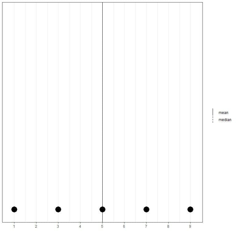
Here we see that both mean and median lines are superimposed over each other.
If we have another set of 5 numbers, 1, 3, 5, 7, 13, the mean = (1+3+5+7+13) /5 = 29/5 = 5.8 and the median will also be 5 because 5 is the central value of this ordered list.
1,3,5,7,13
We can see that from this dot plot.
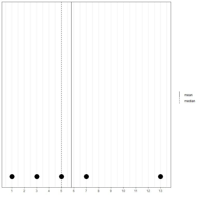
We note that the mean is to the right of (larger than) the median.
If we have another set of 5 numbers, 0.1, 3, 5, 7, 9, the mean = (0.1+3+5+7+9) /5 = 24.1/5 = 4.82 and the median will also be 5 because 5 is the central value of this ordered list.
0.1,3,5,7,9
We can see that from this dot plot.
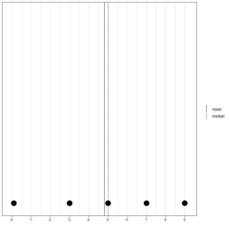
We note that the mean is to the left of (smaller than) the median.
What do we learn from that?
- When the data is evenly spaced (or evenly distributed), the mean and median are nearly the same.
- When there are one or more values that are quite larger than the remaining data, the mean is pulled by them to the right and will be larger than the median. This data is called right-skewed data and we see that in the second set of numbers (1,3,5,7,13).
- When there are one or more values that are quite smaller than the remaining data, the mean is pulled by them to the left and will be smaller than the median. This data is called left-skewed data and we see that in the third set of numbers (0.1,3,5,7,9).
The role of mean value in statistics
The mean is a type of summary statistics used to give important information about a certain data or population. If we have a data set of heights and the mean is 160 cm, so we know that the average value for these heights is 160 cm. This gives us a measure of the center or central tendency of this data.
The mean, in that sense, is often called the expected value of the data. However, the mean will not represent the center of the data when this data is skewed as we see in the examples above. In that case, the median is a better representation of the data center.
For example, the regicor data contains the results of 3 different cross-sectional surveys of individuals from a north-west Spanish province (Girona). Here are the first 100 diastolic blood pressure values (in mmHg) represented as dot plot with their mean (solid line) and median (dashed line).
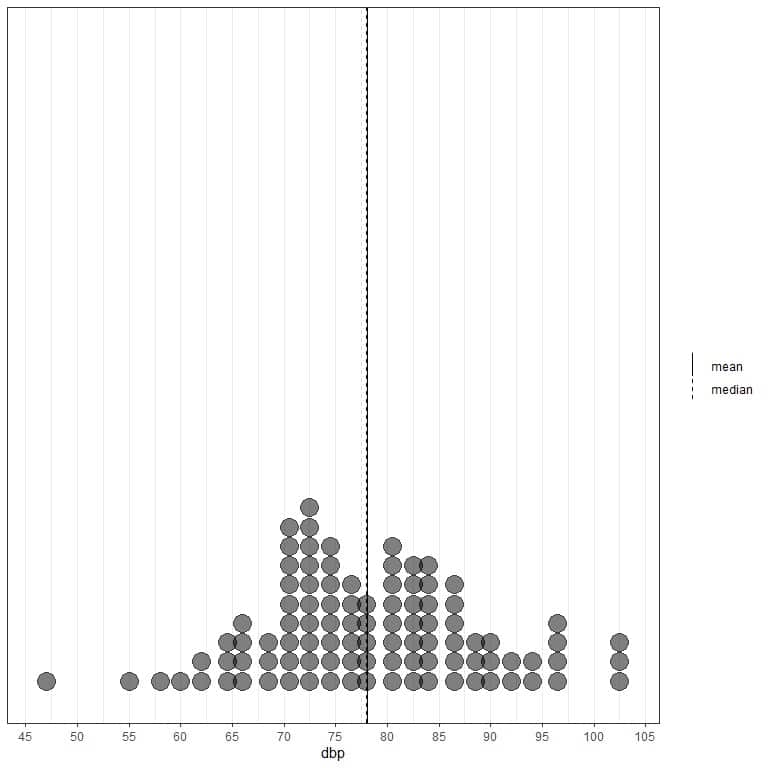
We see that the mean line at 78.08 mmHg (solid line) is nearly superimposed on the median line at 78 mmHg (dashed line) as the data is evenly spaced. There are no observable outliers in this data and this data is called normally distributed data.
If we look at the first 100 physical activity values (in Kcal/week) represented as dot plot with their mean (solid line) and median (dashed line).
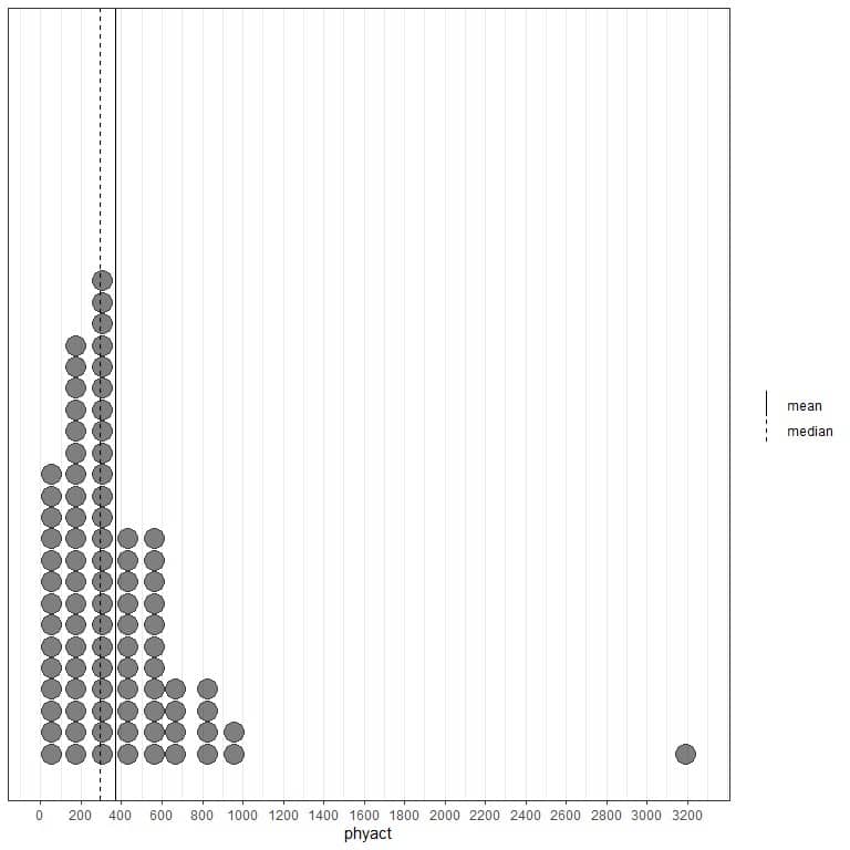
Nearly all the data values are between 0 and 1000. However, the presence of one single outlier value at 3200 has pulled the mean (at 368) to the right of the median (at 292). This data is called right-skewed data.
If we look at the first 100 physical component values represented as a dot plot with their mean (solid line) and median (dashed line).
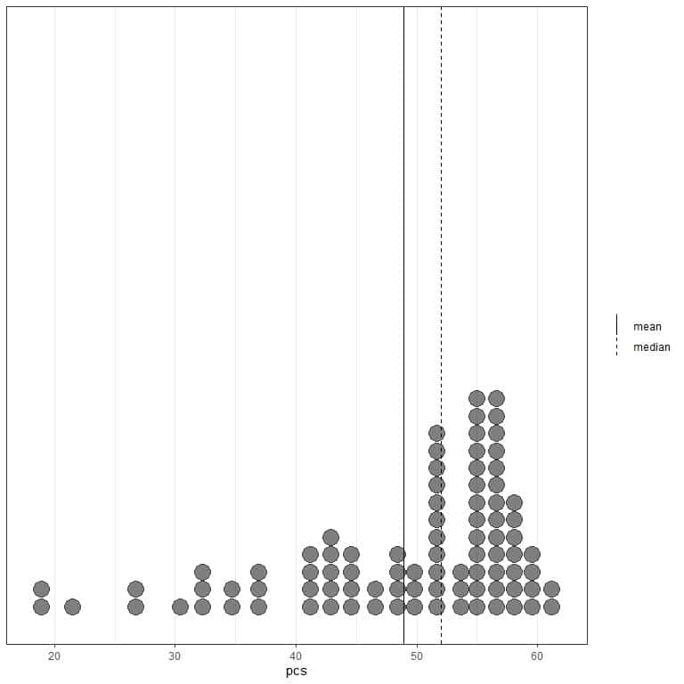
Almost all the data values are between 40 and 60. However, the presence of a few outlier values has pulled the mean (at 48.9) to the left of the median (at 52). This data is called left-skewed data.
One disadvantage of the mean as a summary statistics is that it is sensitive to outliers. Because the mean is sensitive to these outlying values, the mean is not a robust statistics. Robust statistics are measures of data properties that are not sensitive to outliers.
How to find the mean of a set of numbers?
The mean of a certain set of numbers can be found manually (by summing the numbers and dividing by their count) or by mean function from the stats package of R programming language.
Example 1: The following is the age (in years) of 20 different individuals from a certain survey:
70 56 37 69 70 40 66 53 43 70 54 42 54 48 68 48 42 35 72 70
What is the mean of this data?
1.Manual method
Summing the data and dividing by 20 to get the mean
(70+56+37+69+70+40+66+53+43+70+54+42+54+48+68+48+42+35+72+70)/20 = 1107/20 = 55.35
So the mean is 55.35 years
2.mean function of R
The manual method will be tedious when we have a large list of numbers.
The mean function, from the stats package of R programming language, saves our time by giving us the mean of a large list of numbers using only one line of code.
These 20 numbers were the first 20 age numbers of the R built-in regicor dataset from the compareGroups package.
We begin our R session by activating the compareGroups package. The stats package needs no activation as it is part of the base packages in R that are activated when we open our R studio.
Then, we use the data function to import the regicor data into our session.
Finally, we create a vector called x that will hold the first 20 values of the age column (using the head function) from the regicor data and then using the mean function to obtain the mean of these 20 numbers which is 55.35 years.
# activating the compareGroups packages
library(compareGroups)
data(“regicor”)
# reading the data into R by creating a vector that holds these values
x<- head(regicor$age,20)
x
## [1] 70 56 37 69 70 40 66 53 43 70 54 42 54 48 68 48 42 35 72 70
mean(x)
## [1] 55.35
Example 2: The following is the last 20 Ozone measurements (in ppb) from the air quality data. Air quality data contains the daily air quality measurements in New York, May to September 1973.
44 21 28 9 13 46 18 13 24 16 13 23 36 7 14 30 NA 14 18 20
- NA stands for not available
what is the mean of this data?
1.Manual method
- Remove the NA or missing values before summing the data
44 21 28 9 13 46 18 13 24 16 13 23 36 7 14 30 14 18 20
- Now, we have 19 values so we sum these numbers and divide by 19.
(44+21+28+9+13+46+18+13+24+16+13+23+36+7+14+30+14+18+20)/19 = 21.42
so the mean is 21.42 years
2.mean function of R
The same code applies except that we add the argument, na.rm = TRUE, to remove NA values. The mean is 21.42 years as calculated by the manual method.
# loading the air quality data
data(“airquality”)
# reading the data into R by creating a vector that holds these values
x<- tail(airquality$Ozone,20)
x
## [1] 44 21 28 9 13 46 18 13 24 16 13 23 36 7 14 30 NA 14 18 20
mean(x, na.rm = TRUE)
## [1] 21.42105
Example 3: The following is the 50 murder rates per 100,000 population of the 50 states of the USA in 1976
15.1 11.3 7.8 10.1 10.3 6.8 3.1 6.2 10.7 13.9 6.2 5.3 10.3 7.1 2.3 4.5 10.6 13.2 2.7 8.5 3.3 11.1 2.3 12.5 9.3 5.0 2.9 11.5 3.3 5.2 9.7 10.9 11.1 1.4 7.4 6.4 4.2 6.1 2.4 11.6 1.7 11.0 12.2 4.5 5.5 9.5 4.3 6.7 3.0 6.9
what is the mean of this data?
1.Manual method
- We sum the data and divide by 50 to get the mean
(15.1+11.3+7.8+10.1+10.3+6.8+3.1+6.2+10.7+13.9+6.2+5.3+10.3+7.1+2.3+4.5+10.6+ 13.2+2.7+8.5+3.3+11.1+2.3+12.5+9.3+5.0+2.9+11.5+3.3+5.2+9.7+10.9+11.1+1.4+ 7.4+6.4+4.2+6.1+2.4+11.6+1.7+11.0+12.2+4.5+5.5+9.5+4.3+6.7+3.0+6.9)/50 = 368.9/50 = 7.378
so the mean is 7.378 per 100,000 population
2.mean function of R
We create a vector called x that will hold these values then we apply the mean function to get the mean
# reading the data into R by creating a vector that holds these values
x<- c(15.1,11.3,7.8,10.1,10.3,6.8,3.1,6.2,10.7,13.9,6.2,5.3,10.3,7.1,2.3,
4.5,10.6, 13.2,2.7,8.5,3.3,11.1,2.3,12.5,9.3,5.0,2.9,11.5,3.3,5.2,
9.7, 10.9, 11.1, 1.4, 7.4, 6.4, 4.2, 6.1,2.4,11.6,1.7,11.0,12.2,
4.5,5.5,9.5,4.3,6.7,3.0,6.9)
x
## [1] 15.1 11.3 7.8 10.1 10.3 6.8 3.1 6.2 10.7 13.9 6.2 5.3 10.3 7.1 2.3
## [16] 4.5 10.6 13.2 2.7 8.5 3.3 11.1 2.3 12.5 9.3 5.0 2.9 11.5 3.3 5.2
## [31] 9.7 10.9 11.1 1.4 7.4 6.4 4.2 6.1 2.4 11.6 1.7 11.0 12.2 4.5 5.5
## [46] 9.5 4.3 6.7 3.0 6.9
mean(x)
## [1] 7.378
Exercises
1. The following is a dot plot of the state areas (in square miles) of the 50 states of the USA.
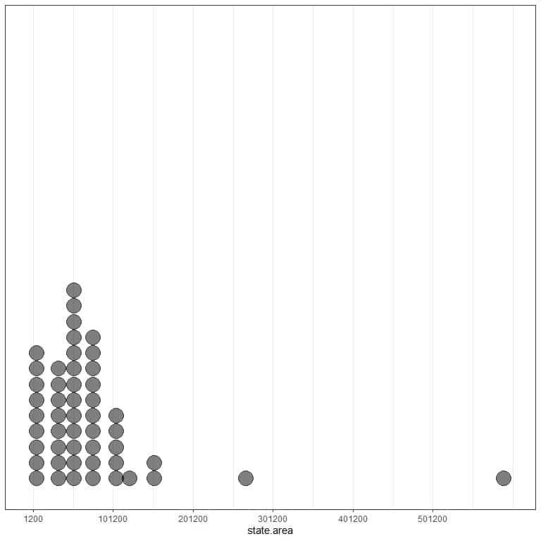
Is this data right or left skewed?
What is the mean and median of this data?
2. The storms data from the dplyr package includes the positions and attributes of 198 tropical storms, measured every six hours during the lifetime of a storm. What is the mean of the wind column (storm’s maximum sustained wind speed in knots)?
3. For the same storms data, what is the mean of the pressure column (Air pressure at the storm’s center in millibars)?
4. For questions 2 and 3 above, which data is right or left-skewed, and why?
5.The air quality data contains Daily air quality measurements in New York, May to September 1973. What is the mean of the Ozone and Solar radiation measurements?
6. Which measurement (Ozone or solar radiation) is right or left-skewed and why?
Answers
1. The states area is a built-in vector in R. From the dot plot, there are some outlying values (areas) on the right side (larger than the rest of other values) so it is right-skewed data.
We can calculate the mean and median directly using R functions
mean(state.area)
## [1] 72367.98
median(state.area)
## [1] 56222
So the mean is 72367.98 square miles which is quite larger than the median that is 56222 square miles. The mean has been pulled up by these larger outlying values that are seen in the dot plot.
2. We begin our session by loading the dplyr package. Then, we load the storms data using the data function. Finally, we calculate the mean using the mean function
# load dplyr package
library(dplyr)
# load storms data
data(“storms”)
# calculate the wind mean
mean(storms$wind)
## [1] 53.495
So the mean is 53.495 knots.
3. The same steps apply.
# load dplyr package
library(dplyr)
# load storms data
data(“storms”)
# calculate the pressure mean
mean(storms$pressure)
## [1] 992.139
So the mean is 992.139 millibars.
4. We calculate the mean and median for each data.
If the mean is larger than the median, so it is right-skewed.
If the mean is smaller than the median, so it is left-skewed.
For the wind data
# load dplyr package
library(dplyr)
# load storms data
data(“storms”)
# calculate the wind mean
mean(storms$wind)
## [1] 53.495
# calculate the wind median
median(storms$wind)
## [1] 45
The mean is 53.495 which is larger than the median (45), so the wind is right-skewed data.
For the pressure data
# load dplyr package
library(dplyr)
# load storms data
data(“storms”)
# calculate the pressure mean
mean(storms$pressure)
## [1] 992.139
# calculate the pressure median
median(storms$pressure)
## [1] 999
The mean is 992.139 which is smaller than the median (999), so the pressure is left-skewed data.
5. The air quality data is a built-in dataset in R. We begin our R session by loading the air quality data using the data function then we calculate the mean for Ozone and solar radiation directly. In both cases, we add the argument, na.rm = TRUE, to exclude the missing values (NA) in these data.
# load the air quality data
data(“airquality”)
# calculate the Ozone mean
mean(airquality$Ozone, na.rm = TRUE)
## [1] 42.12931
# calculate the solar radiation mean
mean(airquality$Solar.R, na.rm = TRUE)
## [1] 185.9315
The mean of ozone measurements is 42.1 ppb, while the mean of solar radiation is 185.9 langleys.
6. To decide which data is right or left-skewed, we calculate the mean and median for each data and compare between them.
For the ozone measurements
# load the air quality data
data(“airquality”)
# calculate the Ozone mean
mean(airquality$Ozone, na.rm = TRUE)
## [1] 42.12931
# calculate the ozone median
median(airquality$Ozone, na.rm = TRUE)
## [1] 31.5
The mean of ozone is 42.1 ppb which is larger than the median (31.5), so it is right-skewed data.
For the solar radiation measurements
# load the air quality data
data(“airquality”)
# calculate the solar radiation mean
mean(airquality$Solar.R, na.rm = TRUE)
## [1] 185.9315
# calculate the solar radiation median
median(airquality$Solar.R, na.rm = TRUE)
## [1] 205
The mean of solar radiation is 185.9 langleys which is smaller than the median (205), so it is left-skewed data.