Mean value theorem – Conditions, Formula, and Examples

The mean value theorem is an important application of derivatives. In fact, it is one of the most important and helpful tools in Calculus, so we need to understand the theorem and learn how we can apply it to different problems.

The mean value theorem helps us understand the relationship shared between a secant and tangent line that passes through a curve.

This theorem also influences the theorems that we have for evaluating first and second derivatives. Knowing about its origin, formula, and application can help us get a head start we need to excel in other Calculus topics.

In fact, the mean value theorem is sometimes coined as “one of the fundamental theorems in differential calculus.” We’ll learn the reason behind this in this article.

What is the mean value theorem?                

According to the mean value theorem, if the function, $f(x)$, is continuous for a closed interval, $[a, b]$, there is at least one point at $x = c$, where the tangent line passing through $f(x)$ will be parallel with the secant line that passes through the points, $(a, f(a))$ and $(b, f(b))$.

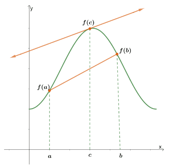
This graph is a good depiction of what we want to show in the mean value theorem. This means that the slopes of this pair of tangent and secant lines are equal, and we can use this to derive the equation we use to find the value of $f’(c)$ – the slope of the tangent line.

Mean value theorem equation

Recall that the slope a line can be calculated using the formula, $m = \dfrac{y_2 – y_1}{x_2 – x _1}$, where $(x_1, y_1)$ and $(x_2, y_2)$ are the two given coordinate pairs. We can apply this to find the slope of the secant line that passes through the points, $(a, f(a))$ and $(b, f(b))$. Equate the result to the tangent line slope, and we’ll have the equation representing the mean value theorem.

\begin{aligned}m_{\text{tangent}} &= f'(c)\\m_{\text{secant}} &= \dfrac{f(b) – f(a)}{b -a}\\\\m_{\text{tangent}} &= m_{\text{secant}}\\f'(c) &= \dfrac{f(b) – f(a)}{b -a} \end{aligned}

This form comes in handy, especially when we want to find the average value of the rate of change of function given an interval we can work on. A special form of the mean value theorem is the Rolles theorem, and this occurs when the value of $f(x)$ is the same when $x = a$ and $x = b$.

Understanding the Rolles theorem

The Rolles theorem is a special application of the mean value theorem. Recall that this theorem states that when $f(x)$ is continuous and differentiable within $[a, b]$, the rate of change between $f(a)$ and $f(b)$ is zero when $f(a) = f(b)$.

We can confirm this by using the mean value theorem:

• Find $f’(c)$ by taking the difference between $f(a)$ and $f(b)$.
• Divide the result by $b – a$.

Since $f(a) = f(b)$, we have zero at the numerator as shown below.

\begin{aligned}f'(c) &= \dfrac{f(b) – f(a)}{b -a}\\&=\dfrac{0}{b -a}\\&= 0 \end{aligned}

This shows that through the mean value theorem, we can confirm that $f’(c)$ or the change rate is equal to $0$ when the function’s end values are equal.

How to use the mean value theorem?                

We’ve shown you how we can use the mean value theorem to prove the Rolles theorem. There are other theorems in differential calculus where we’ll need to apply this important theorem, so we need to learn how we can use this theorem properly.

• Make sure to check if the function is continuous within the interval.
• Check if the function is differentiable within the interval as well.
• Apply the formula to attain our desired result.

For the second bullet, there are two ways for us to check if the function is differentiable. We’ll show you the two ways, and your preferred method will depend on whether you’ve mastered your derivative rules.

As you can see, the second route (using the different derivative rules) is much easier and will help the next step most of the time. For now, let us list down some important derivative rules we might need in this section. Of course, making sure that you know this by heart at this point makes a lot of difference.

These are just some of the rules that might come in handy in our examples but don’t worry, we’ll recall other important derivative rules when the need arises in our discussion.

Once we’ve confirmed that the function is continuous and differentiable, we can then apply the equation representing the mean value theorem.

\begin{aligned}f'(c) &= \dfrac{f(b) – f(a)}{b -a} \end{aligned}

We can then use this to apply the mean value theorem in whatever problem we’re given and derive the output we’re being asked.

Using the mean value theorem to prove a corollary

We can try using the mean value theorem to prove important corollaries. Why don’t we prove the corollary about increasing and decreasing functions?

Let’s say we have a continuous and differentiable function, $f(x)$, within $[a, b]$. The corollary states that:

    i) When $f’(x) >0$, the function is said to be increasing within the given interval.

    ii)When $f’(x) <0$, the function is said to be decreasing within the given interval.

We can use the mean value theorem to prove this by contradiction. We’ll show how i) can be proven, and you can work on your own to show ii).

To prove the first point by contradiction, we can let $a$ and $b$ be part of the interval so that $a < b$ but $f(a) \geq f(b)$. This means that we assume that $f(x)$ is not increasing throughout the interval.  It’s given that $f(x)$ is continuous and differentiable so that we can proceed with the mean value theorem’s equation.

\begin{aligned}f'(c) &= \dfrac{f(b) – f(a)}{b -a} \end{aligned}

We’ve estbalished that $f(a) \geq f(b)$, so we’re expecting $f(b) – f(a)$ to be less than or equation to $0$. In addition, we’ve assumed that $a <b$, so $b -a$ must be greater than zero. Let’s observe the nature of $f’(c)$ given our assumptions.

\begin{aligned}f'(c) &= \dfrac{f(b) – f(a)}{b -a} \\&\leq 0\end{aligned}

But, we want the derivative to be greater than zero, so for this this statement is a contradiction. For $f(x) >0 $, we’ll need $f(b) \geq f(a)$, so $f(x)$ will have to be an increasing function.

This is just one of the many corollaries and theorems that rely on the mean value theorem. This shows how important it is for us to master this theorem and learn the common types of problems we might encounter and require to use the mean value theorem.

Example 1

If $c$ is within the interval, $[2, 4]$, find the value of $c$ so that $f’(c)$ represents the slope within the endpoints of $ y= \dfrac{1}{2}x^2$.

Solution

The function, $y = \dfrac{1}{2}x^2$ is continuous throughout the the interval, $[2, 4]$. We want to find the value of $f’(c)$ to be within $[2, 4]$. Before we can find the value of $c$, we’ll have to confirm that the function is differentiable. In general, quadratic expressions are differentiable, and we can confirm $y = \dfrac{1}{2}x^2$’s nature by either:

• Evaluating limit of the expression,$\lim_{h\rightarrow 0} \dfrac{f(x +h) – f(x)}{h}$, where $f(x + h) = \dfrac{1}{2}(x + h)^2$ and $f(x) = \dfrac{1}{2}x^2$.
• Taking the derivative of $y = \dfrac{1}{2}x^2$ using the power and constant rule.

Just for this example, we can you both approaches – but for the rest, we’ll stick with finding the derivatives and you’ll see why.

See how using limits to confirm that a given function is differentiable is very tedious? This is why it pays to use the derivative rules you’ve learned in the past to speed up the process.  From the two, we have $f’(x) = x$, so this means that $f’(c)$ is equal to $c$.

Using the mean value theorem’s equation, $f'(c) = \dfrac{f(b) – f(a)}{b -a}$, we can replace $f’(c)$ with $c$. We can use the intervals, $[2, 4]$, for $a$ and $b$, respectively.

Let’s use these values into the equation we’re given to find the value of $c$.

\begin{aligned}f'(c) &= \dfrac{f(b) – f(a)}{b -a}\\c &= \dfrac{8 – 2}{4 – 2}\\c &= \dfrac{6}{2}\\c&=3\end{aligned}

This means that for $c$ to be within the interval and still satisfy the mean value theorem, $c$ must be equal to $3$.

Example 2

Let’s say that we have a differentiable function, $f(x)$, so that $f’(x) \leq 4$ for all values of $x$. What is largest value that is possible for $f(18)$ if $f(12) = 30$?

Solution

We are given the following values from the problem:

• $a = 12$, $f(12) = 30$
• $b = 18$, $f(18) = ?$

From the mean value theorem, we know that there exists $c$ within the interval of $x \in [12, 18]$, so we can use the mean value theorem to find the value of $f(12)$.

\begin{aligned}f'(c) &= \dfrac{f(b) – f(a)}{b -a}\\a&= 12\\b&=18\\\\f'(c) &= \dfrac{f(18)- f(12)}{18 – 12}\\&= \dfrac{f(18) – 30}{6}\end{aligned}

Let’s isolate $f(18)$ on the left-hand side of the equation, as shown below.

\begin{aligned}f'(c) \cdot {\color{green} 6}&= \dfrac{f(18)- 30}{6}\cdot {\color{green} 6}\\6f'(c) &= f(18) -30\\f(18) &=6f'(c) + 30 \end{aligned}

Although the value of $c$ and $f’(c)$ are not given, we know the fact that $f’(x) \leq 4$ for all values of $x$, so we’re sure that $f(c) \leq 4$. Let’s use this to rewrite the relationship of $f(18)$ and $f(c)$ in terms of an inequality.

\begin{aligned}f(18) &= 6f'(c)  + 30\\ f'(c) &\leq 4\\\\f(18) &\leq 6(4) + 30\\f(18) &\leq 24 + 30\\f(18) &\leq 54\end{aligned}

This means that the maximum possible value for $f(18)$ is $54$.

Example 3

Verify that the function, $f(x) = \dfrac{x}{x – 4}$, satisfies the conditions of the mean value theorem on the interval $[-2, 2]$ and then determine the value/s, $c$, that can satisfy the conclusion of the theorem.

Solution

When given a rational function, it’s important to see if the interval is within its larger domain to confirm continuity. For $f(x) = \dfrac{x}{x – 4}$, we can see that as long as $x \neq 4$, all values of $x$ are valid. This means that $f(x)$ is continuous within the interval, $[-2, 2]$.

Now, we can find the derivative of $f(x) = \dfrac{x}{x – 4}$ and confirm its differentiability. We can begin by using the quotient rule, $\dfrac{d}{dx} \left[\dfrac{f(x)}{g(x)}\right] =\dfrac{g(x)f'(x) -f(x) g'(x)}{[g(x)]^2}$.

\begin{aligned}\dfrac{d}{dx} \dfrac{x}{x – 4} &= \dfrac{(x -4)\dfrac{d}{dx}x – x \dfrac{d}{dx} (x -4)}{(x -4)^2}\\&=\dfrac{(x – 4)(1) – x(1 – 0)}{(x – 4)^2}\\&= \dfrac{x – 4 – x}{(x – 4)^2}\\&= -\dfrac{4}{(x – 4)^2}\end{aligned}

We can see that it’s possible for us to find the derivative of $f(x)$ and with this, we have $f’(c) = -\dfrac{4}{(c – 4)^2}$.

We’ve shown that $f(x)$ meets the mean value theorem’s conditions, so we can use the concluding equation to find $c$.

• We can let $a = -2$ and $b = 2$, so we can substitute these values into $f(x)$ to find $f(-2)$ and $f(2)$.
• On the left-hand side of the equation, we can then replace $f’(c)$ with $-\dfrac{4}{(c – 4)^2}$.

\begin{aligned}f(-2)&=\dfrac{-2}{-2 – 4}\\&= \dfrac{1}{3}\\f(2) &= \dfrac{2}{2 – 4}\\&=-1\\\\f'(c) &= \dfrac{f(b) – f(a)}{b – a}\\-\dfrac{4}{(c -4)^2} &= \dfrac{-1 – \dfrac{1}{3}}{2 – (-2)}\\-\dfrac{4}{(c – 4)^2} &= \dfrac{-5 – (-1)}{5 – 2}\\-\dfrac{4}{(c – 4)^2}&= -\dfrac{1}{3}\end{aligned}

Cross-multiply then isolate $(c – 4)^2$ on one side of the equation. Solve for $c$ and only take note of the root of $c$ that will be within the interval of $[-2, 2]$.

\begin{aligned}-\dfrac{4}{(c -4)^2}&= -\dfrac{1}{3}\\12 &= (c – 4)^2\\c -4 &= \pm \sqrt{12}\\c&= 4 + 2\sqrt{3}\\&\approx 7.46\\c&= 4 – 2\sqrt{3}\\ &\approx 0.54\end{aligned}

This means that $c$ is equal to $4- 2\sqrt{3}$ or approximately, $0.54$.

Example 4

Verify that the function, $f(x) = \dfrac{x^4}{2 – \sqrt{x}}$, satisfies the conditions of the mean value theorem on the interval $[1, 4]$ and then determine the value/s, $c$, that can satisfy the conclusion of the theorem.

Solution

First, let’s check if the function is continuous before we apply the mean value theorem. We can equate the denominator, $2 – \sqrt{x}$, to check for any restrictions on the function. Once we have the restricted values for $x$, check if these values are within the interval, $[1, 4]$.

\begin{aligned}2 – \sqrt{x} &\neq 0\\\sqrt{x} &\neq 2\\x&\neq 4\end{aligned}

This means that as long as the interval does not contain $x = 4$ within it, the function can be considered continuous for the said interval. Since $ 4 \in [1, 4]$, $f(x)$ is not continuous within the interval.

Hence, we can’t apply the mean value theorem for this problem since it is not continuous within the interval.

This problem is a good example of why we must always ensure the function meets the conditions for us to apply the mean value theorem.

Example 5

Verify that the function, $f(x) = 2x + \sqrt{x – 4}$, satisfies the conditions of the mean value theorem on the interval $[4, 8]$ and then determine the value/s, $c$, that can satisfy the conclusion of the theorem.

Solution

Since we have a radical expression for $f(x)$, we have to ensure that the restricted values are outside the interval, $[4, 8]$. To check for restrictions, we have to ensure that $x – 4$ is greater than or equal to $0$.

\begin{aligned}x – 4 \geq 0 \\x \geq 4\end{aligned}

Since $x \geq 4$ and $x\in [4, 8]$, we can see that the function remains continuous within our given interval. This means that we can then find the derivative of the equation.

To do so, recall that $\sqrt{b} = b^{\frac{1}{2}}$, so we can rewrite $f(x)$ using this property to differentiate it faster.

• Apply the sum rule to differentiate the two terms, first making the process easier.
• Use the power rule to find the derivative of $2x$ and $\sqrt{x – 4} = (x – 4)^{\frac{1}{2}}$.

\begin{aligned} \dfrac{d}{dx} 2x + \sqrt{x – 4} &= \dfrac{d}{dx} 2x + \dfrac{d}{dx} \sqrt{x – 4}\\&= 2\dfrac{d}{dx} x + \dfrac{d}{dx} (x- 4)^{\frac{1}{2}}\\ &=2(1) + \dfrac{1}{2}(x – 4)^{1/2 – 1}\\&= 2 + \dfrac{1}{2} (x-4)^{-\frac{1}{2} }\\&= 2 + \dfrac{1}{2\sqrt{x – 4}}\end{aligned}

From this, we can say that the function is continuous and differentiable, so we can confirm that the conditions for the mean value theorem have been met.

Now that we have the expression for $f’(x)$, what we can do is find $f(4)$ and $f(8)$ then apply the mean value theorem’s equation.

\begin{aligned}f(4)&=2(4) + \sqrt{4 – 4}\\&=8 \\f(8)&=2(8) + \sqrt{8 – 4}\\&= 18 \\\\f'(c) &= \dfrac{f(b) – f(a)}{b – a}\\2 + \dfrac{1}{2\sqrt{c -4}} &= \dfrac{18 – 8}{8 – 4}\\2 + \dfrac{1}{2\sqrt{c -4}} &= \dfrac{10}{4}\\\dfrac{1}{2\sqrt{c -4}}&= \dfrac{1}{2}\end{aligned} Simplify the equation further and square $\sqrt{c – 4}$ once isolated on either side of the equation.

\begin{aligned}\dfrac{1}{\sqrt{c -4}}&= 1\\\sqrt{c – 4} &= 1\\(\sqrt{c – 4} )^2 &= (1)^2\\c – 4 &= \pm 1\\c &= 3, 5\end{aligned}

Choose the value of $c$ that is within the given interval, $[4, 8]$, so we have $c = 5$.

Example 6

Use the mean value theorem to show that $|\sin a – \sin b| \leq |a – b|$ for the interval, $0 \leq a < b \leq 2\pi$.

Solution

The sine function, $f(x) = \sin x $, is known to be continuous within the interval, $[0, 2\pi]$, and we’ve learned in the past that the derivative of $\sin x $ is equal to $\cos x$.

\begin{aligned}f’(x) = \cos x\end{aligned}

This shows that the function $f(x) = \sin x$ meets the conditions for the mean value theorem, so we can use the conclusion to establish the relationship shown below.

\begin{aligned}f'(c) &= \dfrac{f(b) – f(a)}{b – a}\\f'(c) &= \dfrac{\sin b – \sin a}{b – a}\\\cos c &= \dfrac{\sin b – \sin a}{b -a}\end{aligned}

Recall that the values of $\cos c$ will be within the range of $[-1, 1]$, so $|\cos c| \leq 1$. Since $\cos c$ is equal to $\dfrac{\sin b – \sin a}{b – a}$ using the mean value theorem, we have the following inequality:

\begin{aligned}\cos c &= \dfrac{\sin b – \sin a}{b -a}\\|\cos c| &= \left|\dfrac{\sin b – \sin a}{b -a}\right|&\leq 1\end{aligned}

Let’s focus on the inequality, $ \left|\dfrac{\sin b – \sin a}{b -a}\right| \leq 1$.

\begin{aligned}\left|\dfrac{\sin b – \sin a}{b -a}\right|&\leq 1\\\dfrac{|\sin b – \sin a}{|b -a|} &\leq 1\\|\sin b – \sin a| &\leq |b – a|\end{aligned}

This confirms the statement we want to prove:$|\sin b – \sin a| \leq |b – a|$. Hence, we’ve shown how it’s possible to prove mathematical statements using the mean value theorem.

Practice Questions

1. If $c$ is within the interval, $[4, 8]$, find the value of $c$ so that $f’(c)$ represents the slope within the endpoints of $ y= -2x^3$.
2. Let’s say that we have a differentiable function, $f(x)$, so that $f’(x) \leq 12$ for all values of $x$. What is largest value that is possible for $f(20)$ if $f(15) = 60$?
3. Verify that the function, $f(x) = \dfrac{2x}{x – 3}$, satisfies the conditions of the mean value theorem on the interval $[-1, 1]$ and then determine the value/s, $c$, that can satisfy the conclusion of the theorem.
4. Verify that the function, $f(x) = 3x + \sqrt{x – 9}$, satisfies the conditions of the mean value theorem on the interval $[9, 15]$ and then determine the value/s, $c$, that can satisfy the conclusion of the theorem.
5. Verify that the function, $f(x) = \dfrac{x^3}{3 – 3\sqrt{x}}$, satisfies the conditions of the mean value theorem on the interval $[1, 5]$ and then determine the value/s, $c$, that can satisfy the conclusion of the theorem.

Answer Key

1. $\dfrac{4\sqrt{21}}{3} \approx 6.11$
2. $120$
3. $3 – 2\sqrt{2} \approx 0.17$
4. $\dfrac{21}{2} = 10.5$
5. The function is not continuous within the interval, so the mean value theorem can’t be applied.

Images/mathematical drawings are created with GeoGebra.