JUMP TO TOPIC
Median statistics – Explanation & Examples
 The definition of the median is:
“Median is the middle number in a sorted data values”
In this topic, we will discuss the median from the following aspects:
- What is the median in statistics?
- The role of the median value in statistics
- How to find the median of a set of numbers?
- Exercises
- Answers
What is the median in statistics?
The median is the value that halves a set of sorted data values equally. In other words, it is the middle value of a data set
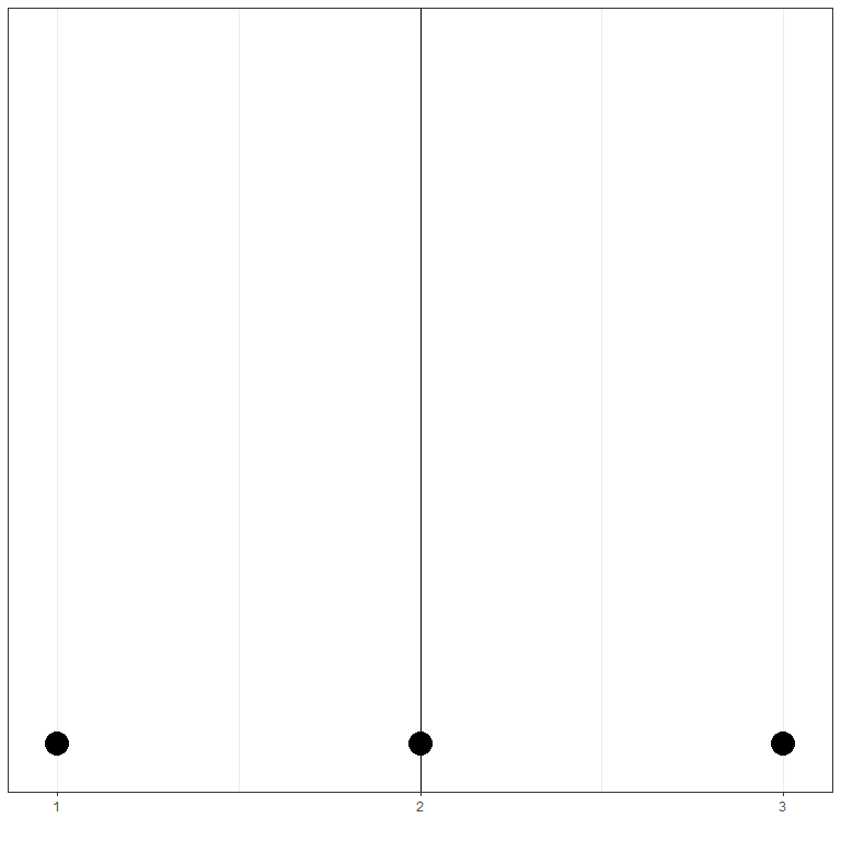
If we have an odd set of numbers, we sort them first, and then the median is the middle number with an equal amount of numbers above and below it. For example, if we have a set of numbers, 1,2,3, the median will be 2 because there is one number below it (1) and one number above it (3).
This can be easily shown if we plot a simple dot plot of this data:
Let’s look at another example, if we have another set of numbers, 1, 3, 5, 6, 8, 10, 11, the median will be 6 because 6 has 3 numbers below it (1,3,5) and 3 numbers above it (8,10,11).
If we have an unsorted list of numbers, we should sort them first and then pick the middle value as the median.
For example, if we have a data set of heights for 17 Spanish individuals, in centimeters, these heights are:
160.0 163.0 170.0 147.0 164.0 160.0 160.0 163.0 160.0 167.0 150.0 156.0 157.0 163.0 162.0 155.0 158.5
We sort this data first to give this
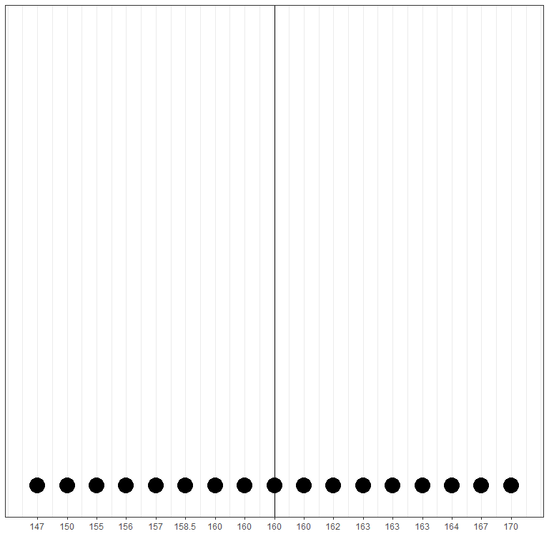
147.0 150.0 155.0 156.0 157.0 158.5 160.0 160.0 160.0 160.0 162.0 163.0 163.0 163.0 164.0 167.0 170.0
The median will be 160 as there are 8 numbers above it and 8 numbers below it.
147.0 150.0 155.0 156.0 157.0 158.5 160.0 160.0 160.0 160.0 162.0 163.0 163.0 163.0 164.0 167.0 170.0
By plotting the data as a dot plot, we could easily see that the median is 160
But what about an even list of numbers? In that case, the numbers are sorted and the middle two numbers are selected. Then, these two numbers are added together and divided by two to get the median. Therefore, the median may be a different number not present in the original data.
For example, if we have a data set of heights for 18 Spanish individuals, in centimeters, these heights are:
160.0 163.0 170.0 147.0 164.0 160.0 160.0 163.0 160.0 167.0 150.0 156.0 157.0 163.0 162.0 155.0 158.5 172.0
We sort this data to give this
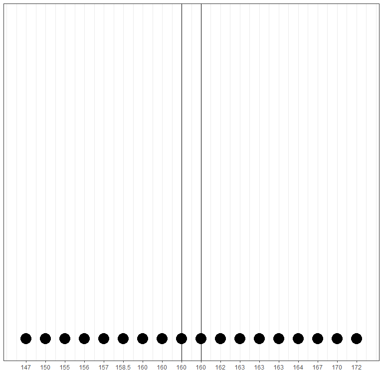
147.0 150.0 155.0 156.0 157.0 158.5 160.0 160.0 160.0 160.0 162.0 163.0 163.0 163.0 164.0 167.0 170.0 172.0
The middle two points are 160,160 as there are 8 numbers above them and 8 numbers below them.
147.0 150.0 155.0 156.0 157.0 158.5 160.0 160.0 160.0 160.0 162.0 163.0 163.0 163.0 164.0 167.0 170.0 172.0
So the median = (160+160)/2 = 160
By plotting the data as a dot plot, we could easily see that the middle pair is 160 and 160. So the median will be (160+160)/2 = 160 also.
Another example, if we have a data set of weights for 10 Spanish individuals, in kilograms, these weights are:
64.0 67.0 70.0 68.0 79.2 53.0 62.0 79.0 66.0 65.0
We sort this data to give this
53.0 62.0 64.0 65.0 66.0 67.0 68.0 70.0 79.0 79.2
The middle two points are 66,67 as there are 4 numbers above them and 4 numbers below them.
53.0 62.0 64.0 65.0 66.0 67.0 68.0 70.0 79.0 79.2
So the median = (66+67)/2 = 66.5 Kg
By plotting the data as a dot plot, we could easily see that the middle pair is 66 and 67. So the median will be (66+67)/2 = 66.5 kg which is a different value not present in the original data values.
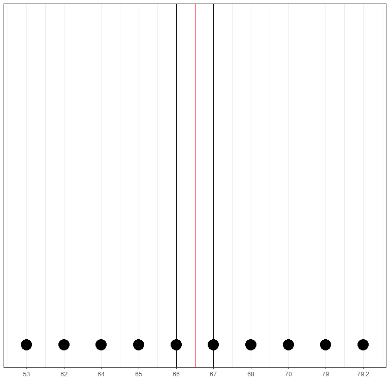
Here the red line represents the median value that is the middle value between 66 and 67 or 66.5 kg.
The role of the median value in statistics
The median is a type of summary statistics used to give important information about a certain data or population.
For the example of the data set of heights, the median is 160 cm, so we know that central height value for these 17 Spanish individuals. This gives us a measure of the location of this data.
If we have another two data sets of heights for another 17 Spanish individuals, and whose median is 164 cm and 186 respectively. Therefore, we can conclude that the third group has the longest heights among the three groups without even looking at its values.
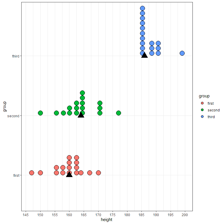
The black triangle represents the median for each group. Here, we see that the third group has the longest heights (blue dots) and this is translated into a median that is shifted more to the right as it represents the location of the data.
The advantage of the median as a summary statistics is that it gives the location without affected by the extreme values or outliers. Outliers may not be trusted in some cases, for example, due to measurement errors. Also, there are many cases where the data naturally has outliers, for example, the income data where most individuals have low or moderate income and there are few individuals with extremely large incomes. Median, as not affected by these outlying values, is a type of robust statistics.
To show that the median is not affected by outliers. Let’s consider this dataset of salaries of 5 managers in the USA, in $1000:
30,50,55,60,70
Here we have the salaries of 5 managers with nearby salaries and the median is $55,000
But if we have another set of 5 salaries with the same values except that the highest salary was $700,000:
30,50,55,60,700
The median will also be $55,000 despite the presence of this outlying salary. This can also be seen in the following figure.
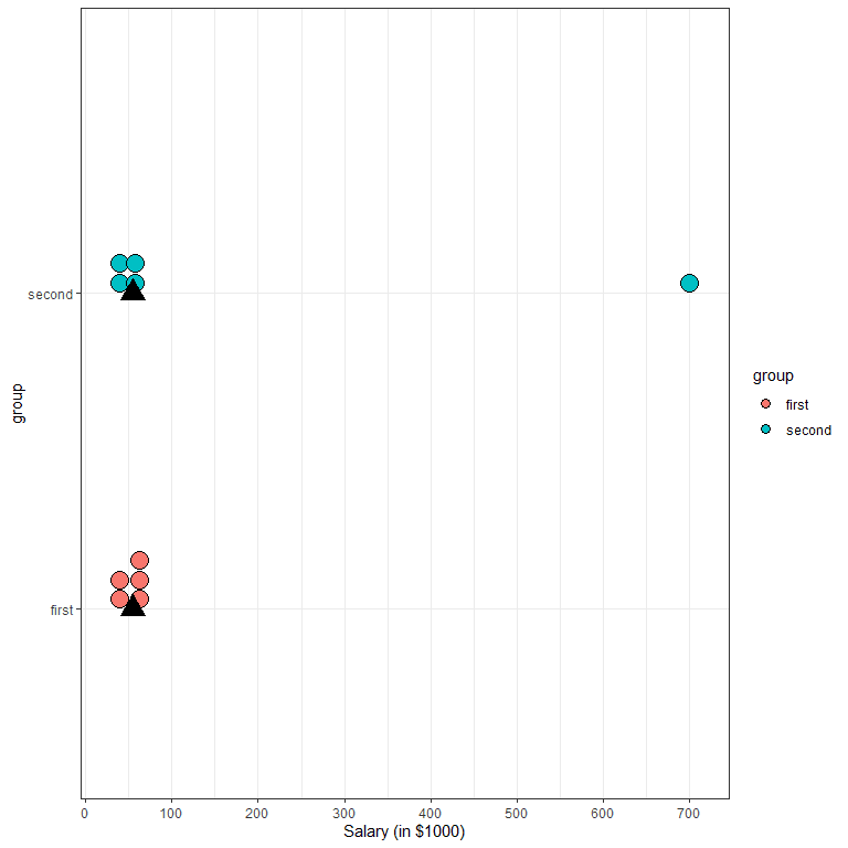
We note that despite the presence of the outlying salary at $700,000 in the second group, the median (represented by black triangles) is still the same for the two groups.
How to find the median of a set of numbers?
The median of a certain set of numbers can be found manually (by the method stated above) or by median function from the stats package of R programming language. If we have an odd list of numbers, the median value is the middle value from the sorted list. If we have an even list of numbers, the median value is the sum of the middle pair divided by two.
Example 1 of an odd list of numbers
The following is the age (in years) of 51 different individuals from a certain survey in Spain:
70 56 37 69 70 40 66 53 43 70 54 42 54 48 68 48 42 35 72 70 70 48 56 74 57 52 58 62 56 68 70 46 35 56 50 48 47 60 63 71 43 65 38 64 73 54 67 58 62 70 58
What is the median of this data?
1.Manual method
- sorting the data
35 35 37 38 40 42 42 43 43 46 47 48 48 48 48 50 52 53 54 54 54 56 56 56 56 57 58 58 58 60 62 62 63 64 65 66 67 68 68 69 70 70 70 70 70 70 70 71 72 73 74
- Pick the middle value =57 years as there are 25 values below it and 25 values above it.
35 35 37 38 40 42 42 43 43 46 47 48 48 48 48 50 52 53 54 54 54 56 56 56 56 57 58 58 58 60 62 62 63 64 65 66 67 68 68 69 70 70 70 70 70 70 70 71 72 73 74
So the median is 57 years
2.median function of R
The manual method will be tedious when we have a large list of numbers as it requires sorting of the numbers then selecting the middle value or the middle pair. The median function, from the stats package of R programming language, saves our time by giving us the median of a large list of numbers using only one line of code.
These 51 numbers were the first 51 age numbers of the R built-in regicor dataset from the compareGroups package.
We begin our R session by activating the compareGroups package. The stats package needs no activation as it is part of the base packages in R that are activated when we open our R studio. Then, we use the data function to import the regicor data into our session.
Finally, we create a vector called x that will hold the first 51 values of the age column (using the head function) from the regicor data and then using the median function to obtain the median of these 51 numbers which is 57 years.
# activating the compareGroups packages
library(compareGroups)
data(“regicor”)
# reading the data into R by creating a vector that holds these values
x<- head(regicor$age,51)
x
## [1] 70 56 37 69 70 40 66 53 43 70 54 42 54 48 68 48 42 35 72 70 70 48 56 74 57
## [26] 52 58 62 56 68 70 46 35 56 50 48 47 60 63 71 43 65 38 64 73 54 67 58 62 70
## [51] 58
median(x)
## [1] 57
Example 2 of an odd list of numbers: The following is the last 21 diastolic blood pressures (dbp) (in mmHg) from regicor data
62 90 106 65 95 88 74 79 85 69 70 73 72 68 89 77 64 80 110 100 65
what is the median of this data?
1.Manual method
- Sorting the data
62 64 65 65 68 69 70 72 73 74 77 79 80 85 88 89 90 95 100 106 110
- Pick the middle value = 77 mmHg as there are 10 values below it and 10 values above it.
62 64 65 65 68 69 70 72 73 74 77 79 80 85 88 89 90 95 100 106 110
2.median function of R
These 21 numbers were the last 21 diastolic blood pressure measurement of the R built-in regicor dataset from the compareGroups package. We apply the same steps except that we create a vector called x that will hold the last 21 values of the diastolic blood pressure column (using the tail function) from the regicor data. The median is 77 mmHg as calculated by the manual method.
# activating the compareGroups packages
library(compareGroups)
data(“regicor”)
# reading the data into R by creating a vector that holds these values
x<- tail(regicor$dbp,21)
x
## [1] 62 90 106 65 95 88 74 79 85 69 70 73 72 68 89 77 64 80 110
## [20] 100 65
median(x)
## [1] 77
Example 3 of an even list of numbers: The following is the last 20 systolic blood pressures (dbp) (in mmHg) from regicor data
138 140 95 170 128 122 117 164 113 100 113 128 135 127 110 112 120 198 155 107
what is the median of this data?
1.Manual method
- Sorting the data
95 100 107 110 112 113 113 117 120 122 127 128 128 135 138 140 155 164 170 198
- Pick the middle pair = (122,127) as there are 9 values below it and 9 values above it.
95 100 107 110 112 113 113 117 120 122 127 128 128 135 138 140 155 164 170 198
- Add these two numbers and divide by two to get the median
(122+127)/2 = 124.5 so the median is 124.5 mmHg
2.median function of R
These 20 numbers were the last 20 systolic blood pressure measurement of the R built-in regicor dataset from the compareGroups package so we use the same method stated above.
# activating the compareGroups packages
library(compareGroups)
data(“regicor”)
# reading the data into R by creating a vector that holds these values
x<- tail(regicor$sbp,20)
x
## [1] 138 140 95 170 128 122 117 164 113 100 113 128 135 127 110 112 120 198 155
## [20] 107
median(x)
## [1] 124.5
Example 4 of an even list of numbers with missing data: The following is the first 20 total cholesterol levels (chol) (in mg/dl) from regicor data
294 220 245 168 NA NA 298 254 194 188 268 116 211 162 209 163 218 238 NA 182
*NA stands for not available
what is the median of this data?
1.Manual method
- Removing the missing values and sorting the remaining data
116 162 163 168 182 188 194 209 211 218 220 238 245 254 268 294 298
- The remaining data is only 17 numbers so we pick the middle value or the median which is 211
116 162 163 168 182 188 194 209 211 218 220 238 245 254 268 294 298
2.median function of R
These 20 numbers were the first 20 total cholesterol measurements of the R built-in regicor dataset from the compareGroups package, so we apply the same steps stated above. In addition, we add the argument, na.rm = TRUE, to this function to remove NA values before calculating the median.
# activating the compareGroups packages
library(compareGroups)
data(“regicor”)
# reading the data into R by creating a vector that holds these values
x<- head(regicor$chol,20)
x
## [1] 294 220 245 168 NA NA 298 254 194 188 268 116 211 162 209 163 218 238 NA
## [20] 182
median(x, na.rm = TRUE)
## [1] 211
Practical Questions
1.The USArrests data contains statistics, in arrests per 100,000 residents for assault, murder, and rape in each of the 50 US states in 1973, what is the median of the murder arrests (Murder column)?
2.For the same USArrests data, what is the median of the Rape arrests (Rape column)?
3.The iris data set gives the measurements in centimeters of the variables sepal length and width and petal length and width, respectively, for 50 flowers from each of 3 species of iris. The species are setosa, versicolor, and virginica. What is the median of the Sepal length?
4.For the same iris data, what is the median of the petal length?
5.Do the values of the median for sepal length and petal length present in the original data? why or why not?
Answers
1.The USArrests data is a built-in data in R. So we import the data using the data function, create a vector to hold the murder arrests values and use the median function.
data(“USArrests”)
x<-USArrests$Murder
median(x)
## [1] 7.25
So the median is 7.25 murder arrests per 100,000 residents.
2.The same steps apply
data(“USArrests”)
x<-USArrests$Rape
median(x)
## [1] 20.1
So the median is 20.1 rape arrests per 100,000 residents.
3.The iris data is a built-in data in R so the same steps apply.
data(“iris”)
x<-iris$Sepal.Length
median(x)
## [1] 5.8
So the median is 5.8 cm.
4.The same steps apply
data(“iris”)
x<-iris$Petal.Length
median(x)
## [1] 4.35
So the median is 4.35 cm.
5.The median value of the sepal length is 5.8 and it is present in the original data. On the other hand, the median of the petal length is 4.35 which is not present in the original data.
For the sepal length, the middle pair is 5.8, 5.8 so the median is 5.8 also. On the other hand, the middle pair for the petal length is 4.3, 4.4 so the median is 4.35.
Using the sort function of the R programming language, we can select the middle pair by using the square brackets index. The middle pair will have indices of 75 and 76.
# original data
sort(iris$Sepal.Length)
## [1] 4.3 4.4 4.4 4.4 4.5 4.6 4.6 4.6 4.6 4.7 4.7 4.8 4.8 4.8 4.8 4.8 4.9 4.9
## [19] 4.9 4.9 4.9 4.9 5.0 5.0 5.0 5.0 5.0 5.0 5.0 5.0 5.0 5.0 5.1 5.1 5.1 5.1
## [37] 5.1 5.1 5.1 5.1 5.1 5.2 5.2 5.2 5.2 5.3 5.4 5.4 5.4 5.4 5.4 5.4 5.5 5.5
## [55] 5.5 5.5 5.5 5.5 5.5 5.6 5.6 5.6 5.6 5.6 5.6 5.7 5.7 5.7 5.7 5.7 5.7 5.7
## [73] 5.7 5.8 5.8 5.8 5.8 5.8 5.8 5.8 5.9 5.9 5.9 6.0 6.0 6.0 6.0 6.0 6.0 6.1
## [91] 6.1 6.1 6.1 6.1 6.1 6.2 6.2 6.2 6.2 6.3 6.3 6.3 6.3 6.3 6.3 6.3 6.3 6.3
## [109] 6.4 6.4 6.4 6.4 6.4 6.4 6.4 6.5 6.5 6.5 6.5 6.5 6.6 6.6 6.7 6.7 6.7 6.7
## [127] 6.7 6.7 6.7 6.7 6.8 6.8 6.8 6.9 6.9 6.9 6.9 7.0 7.1 7.2 7.2 7.2 7.3 7.4
## [145] 7.6 7.7 7.7 7.7 7.7 7.9
sort(iris$Petal.Length)
## [1] 1.0 1.1 1.2 1.2 1.3 1.3 1.3 1.3 1.3 1.3 1.3 1.4 1.4 1.4 1.4 1.4 1.4 1.4
## [19] 1.4 1.4 1.4 1.4 1.4 1.4 1.5 1.5 1.5 1.5 1.5 1.5 1.5 1.5 1.5 1.5 1.5 1.5
## [37] 1.5 1.6 1.6 1.6 1.6 1.6 1.6 1.6 1.7 1.7 1.7 1.7 1.9 1.9 3.0 3.3 3.3 3.5
## [55] 3.5 3.6 3.7 3.8 3.9 3.9 3.9 4.0 4.0 4.0 4.0 4.0 4.1 4.1 4.1 4.2 4.2 4.2
## [73] 4.2 4.3 4.3 4.4 4.4 4.4 4.4 4.5 4.5 4.5 4.5 4.5 4.5 4.5 4.5 4.6 4.6 4.6
## [91] 4.7 4.7 4.7 4.7 4.7 4.8 4.8 4.8 4.8 4.9 4.9 4.9 4.9 4.9 5.0 5.0 5.0 5.0
## [109] 5.1 5.1 5.1 5.1 5.1 5.1 5.1 5.1 5.2 5.2 5.3 5.3 5.4 5.4 5.5 5.5 5.5 5.6
## [127] 5.6 5.6 5.6 5.6 5.6 5.7 5.7 5.7 5.8 5.8 5.8 5.9 5.9 6.0 6.0 6.1 6.1 6.1
## [145] 6.3 6.4 6.6 6.7 6.7 6.9
# select the middle pair
sort(iris$Sepal.Length)[c(75,76)]
## [1] 5.8 5.8
sort(iris$Petal.Length)[c(75,76)]
## [1] 4.3 4.4