The Poisson Distribution – Explanation & Examples

The definition of the Poisson distribution is:

“The Poisson distribution is a discrete probability distribution that describes the probability of the number of events occurring in a fixed interval.”

In this topic, we will discuss the Poisson distribution from the following aspects:

• What is a Poisson distribution?
• When to use Poisson distribution?
• Poisson distribution formula.
• How to do the Poisson distribution?
• Practice questions.
• Answer key.

What is a Poisson distribution?

The Poisson distribution is a discrete probability distribution that describes the probability of the number of events (discrete random variable) from a random process in a fixed interval.

Discrete random variables take a countable number of integer values and cannot take decimal values. Discrete random variables are usually counts.

The fixed interval can be:

• Time as the number of calls received per hour in a call center or the number of goals per football match.
• Distance as the number of mutations on a strand of DNA per unit length.
• Area as the number of bacteria found per unit area of an agar plate.
• Volume as the number of bacteria found per milliliter of a liquid.

The Poisson distribution is named after the French mathematician Siméon Denis Poisson.

When to use Poisson distribution?

You can apply the Poisson distribution to random processes with a large number of possible events, each of which is rare.

However, the average rate (the average number of events per interval) can be any number and does not always have to be small.

For the Poisson distribution to describe a random process, it must be:

1. The number of events occurring in an interval can take values 0, 1, 2, ….etc. No decimal numbers are allowed because it is a discrete distribution or a count distribution.
2. The occurrence of one event does not affect the probability that a second event will occur. That is, events occur independently.
3. The average rate (the average number of events per interval) is constant and does not change based on time.
4. Two events cannot occur at the same time. It means that at each sub-interval, either an event occurs or not.

– Example 1

Data from a certain call center shows a historical average of 10 calls received per hour. What is the probability of receiving 0, 10, 20, or 30 per hour in this center?

We can use the Poisson distribution to describe this process because:

1. The number of calls per hour can take values 0, 1, 2, ….etc. No decimal numbers can occur.
2. The occurrence of one event does not affect the probability that a second event will occur. There is no reason to expect a caller to affect the chances of another person calling, and so the events occur independently.
3. We may assume the average rate (the number of calls per hour) to be constant.
4. Two calls cannot occur at the same time. It means that at each sub-interval, like second or minute, either a call occurs or not.

This process is not a perfect fit for the Poisson distribution. For example, the average rate of calls per hour may decrease in the night hours.

Practically speaking, the process (the number of calls per hour) is close to the Poisson distribution and can be used to describe the process’s behavior.

Using the Poisson distribution can help us to calculate the probability of 0,10,20 or 30 calls per hour:

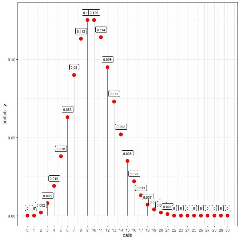The probability of zero calls per hour = 0%.

The probability of 10 calls per hour = 0.125 or 12.5%.

The probability of 20 calls per hour = 0.002 or 0.2%.

The probability of 30 calls per hour = 0%.

We see that 10 calls have the highest probability, and as we move away from 10, the probability fades away.

We can connect the points to draw a curve:

The average rate of 10 calls per hour has the highest probability (curve peak). As we move away from 10, the probability fades away.

The average rate (the average number of events per interval) can take a decimal value. In that case, the number of events with the highest probability will be the nearest integer to the average rate, as we will see in the following example.

– Example 2

Data from the maternity ward in a certain hospital shows 2372 babies born in this hospital in the last year. The average per day = 2372/365 = 6.5.

What is the probability that 10 babies will be born in this hospital tomorrow?

How many days of the next year that 10 babies per day will be born in this hospital?

The number of babies born per day in this hospital can be described using the Poisson distribution because:

1. The number of babies born per day can take values 0, 1, 2, ….etc. No decimal numbers can occur.
2. The occurrence of one event does not affect the probability that a second event will occur. We do not expect that a newborn baby will affect another baby’s chances to be born in that hospital unless the hospital is full, so the events occur independently.
3. The average rate (the number of babies born per day) may be assumed to be constant.
4. Two babies cannot be born at the same time. It means that either a baby is born or not at each sub-interval, like second or minute.

The number of babies born per day is close to the Poisson distribution. We can use the Poisson distribution to describe the process’s behavior.

The Poisson distribution can help us to calculate the probability of 10 babies born per day:

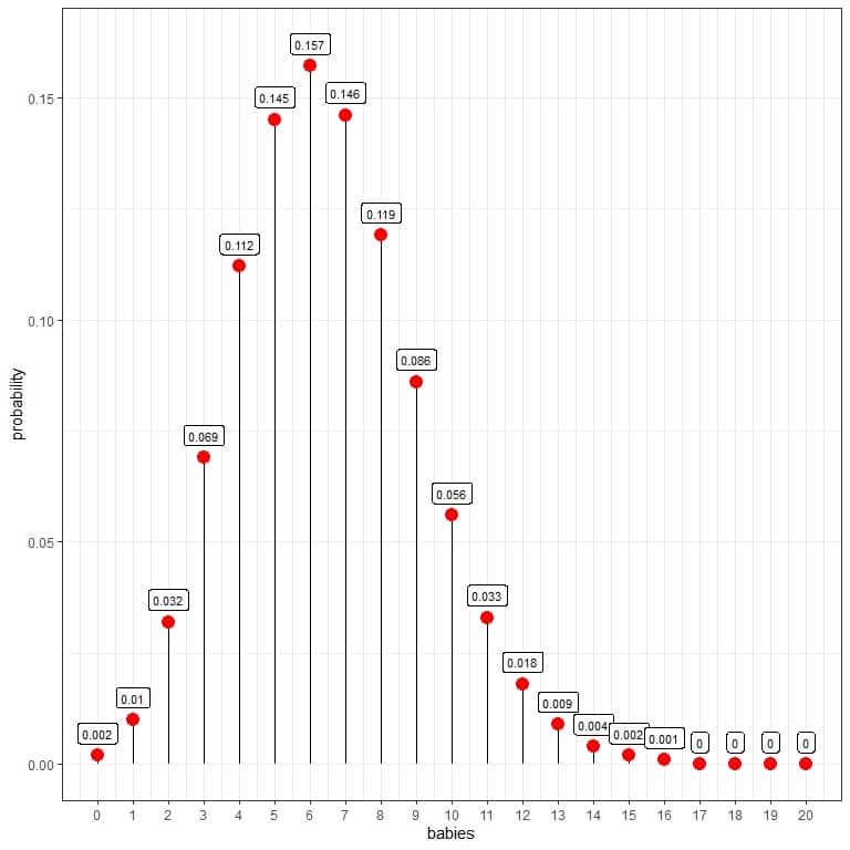The probability of 10 babies born per day = 0.056 or 5.6 %.

We see that 6 babies have the highest probability.

When the number of babies is larger than 16, the probability is very small and can be considered zero.

We can connect the points to draw a curve:

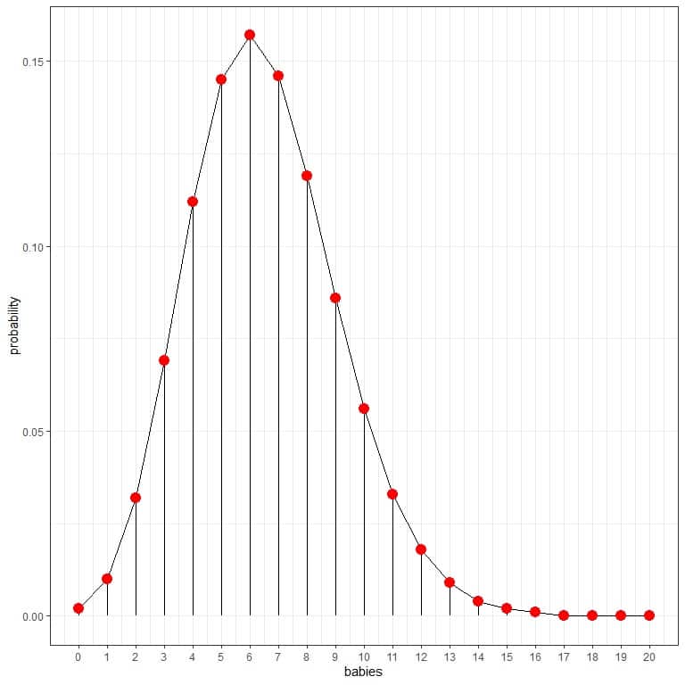
The 6 babies per day have the highest probability (curve peak), and as we move away from 6, the probability fades away.

1. To know the number of days in the next year, this hospital will expect a different number of births.

We construct a table with each outcome (number of babies) and its probability.
babies probability

2. Add another column for the expected days. Fill that column by multiplying each probability value by the number of days in a year (365).

We expect that about 20 days out of the total 365 days of the next year, this hospital will deliver 10 births per day.

– Example 3

The average number of goals in a World Cup soccer match is approximately 2.5.

The number of goals per football match can be described using the Poisson distribution because:

1. The number of goals per football match can take values 0, 1, 2, ….etc. No decimal numbers can occur.
2. The occurrence of one event (goal) does not affect the probability that a second event will occur, and so the events occur independently.
3. The average rate (the number of goals per match) may be assumed to be constant.
4. Two goals cannot occur at the same time. It means that at each sub-interval of the match, like second or minute, either a goal occurs or not.

The number of goals per match is close to the Poisson distribution. We can use the Poisson distribution to describe the process’s behavior.

The Poisson distribution can help us to calculate the probability of each number of goals in a football match:

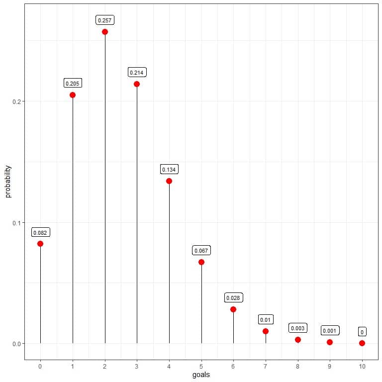We see that 2 goals per match have the highest probability = 0.257 or 25.7%.
Examples of 2 goals per match are a score of 2-0 or 1-1.

When the number of goals is larger than 9, the probability is very small and can be considered zero.

We can connect the points to draw a curve:

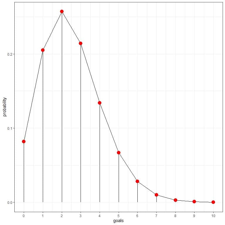
The 2 goals per match have the highest probability (curve peak), and as we move away from 2, the probability fades away.

64 matches are played in World Cup soccer. We can use the Poisson distribution to calculate the number of matches that will likely contain the different number of goals:

1. We construct a table with each outcome (number of goals) and its probability.
goals probability

2. Add another column for the expected matches.

Fill that column by multiplying each probability value by the number of matches in World Cup soccer (64).

We are expecting:

About 6 matches will contain no goals.

About 13 matches will contain 1 goal.

About 16 matches will contain 2 goals.

About 13 matches will contain 3 goals, and so on.

3. We can add another column for the observed number of goals in the World Cup soccer of 2018 in Russia to see how closely the Poisson distribution predicts the number of goals:

We see that the expected number of matches found by Poisson distribution is near the observed number of matches having these goals.

The Poisson distribution is good at describing this process behavior. Similarly, you can use it to predict the number of goals per match in the next World Cup of 2022.

Poisson distribution formula

If the random variable X follows the Poisson distribution with λ average number of events per fixed interval, the probability of getting exactly k events in this fixed interval is given by:

f(k,λ)=”P(k events in the interval)”=(λ^k.e^(-λ))/k!

where:

f(k,λ) is the probability of k events per fixed interval.

λ is the average number of events per fixed interval.

e is a mathematical constant approximately equal to 2.71828.

k! is the factorial of k and equals to k X (k-1) X (k-2) X….X1.

How to do the Poisson distribution?

To calculate the Poisson distribution for the number of events in a fixed interval, we only need the average number of events in a fixed interval.

– Example 1

Data from a certain call center shows a historical average of 10 calls received per hour. Assuming that this process follows the Poisson distribution, what is the probability that the call center will receive 0,10,20, or 30 calls per hour?

1. Construct a table for the different number of events:

2. Add another column named “average^calls” for the λ^k term. λ is the average events number = 10 and k = 0,10,20,30.

The first value is 10^0 = 1.

The second value is 10^10 = 1 X 10^10 = 1e+10 in a scientific notation.

The third value is 10^20 = 1 X 10^20 = 1e+20 in a scientific notation.

The fourth value is 10^30 = 1 X 10^30 = 1e+30 in a scientific notation.

3. Add another column named “multiplied average^calls” for the multiplication of average^calls by e^(-λ) = 2.71828^-10.

4. Add another column named “probability” by dividing each value of the “multiplied average^calls” by factorial calls.

For 0 calls, the factorial = 1.

For 10 calls, the factorial = 10X9X8X7X6X5X4X3X2X1 = 3628800.

For 20 calls, the factorial = 20X19X18X17X16X15X14X13X12X11X10X9X8X7X6X5X4X3X2X1 = 2.432902e+18, and so on.

5. With similar calculations, we can calculate the probability of the different number of calls per hour, from 0 to 30, as we see in the following table and plot:

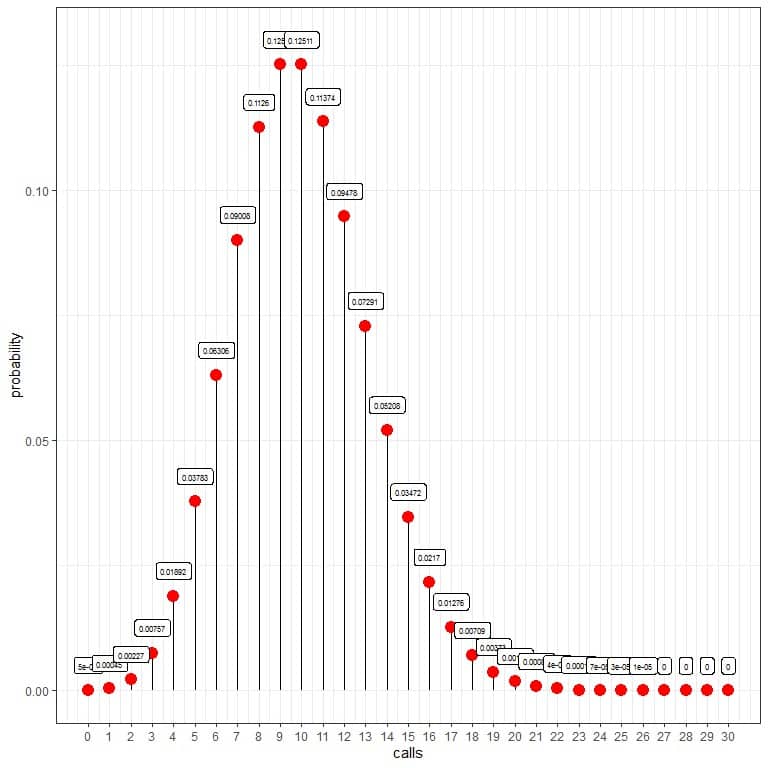
The probability of zero calls per hour = 0.00005 or 0.005%.

The probability of 10 calls per hour = 0.12511 or 12.511%.

The probability of 20 calls per hour = 0.00187 or 0.187%.

The probability of 30 calls per hour = 0%.

We see that 10 calls have the highest probability, and as we move away from 10, the probability fades away.

We can connect the points to draw a curve:

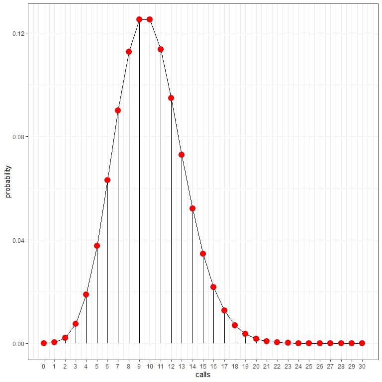
We can use these probabilities to calculate how many hours per day are expected to receive these calls.

We multiply each probability by 24 as the day contains 24 hours.

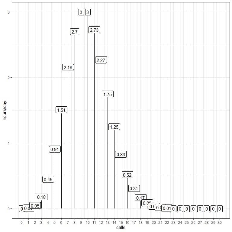
We are expecting 3 hours of the day to contain 10 calls per hour.

– Example 2

In the following table and plot, we will use the Poisson distribution to calculate the probability of the different number of calls per hour from 0 to 30 if the average calls were 2 calls/hour, 10 calls/hour, or 20 calls/hour:

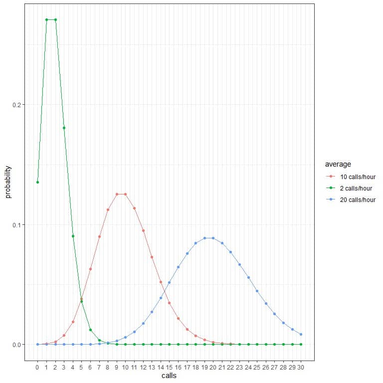
Every curve peak corresponds to the average value for that curve.

The curve for the average 2 calls/hour (green curve) has a peak at 2.

The curve for the average 10 calls/hour (red curve) has a peak at 10.

The curve for the average 20 calls/hour (blue curve) has a peak at 20.

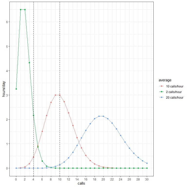
We can use these probabilities to calculate how many hours per day are expected to receive these calls when the average is 2 calls/hour, 10 calls/hour, or 20 calls/hour.

We multiply each probability by 24 as the day contains 24 hours.

For example:

• We expect 2 hours of the day to contain 4 calls per hour when the average is 2 calls/hour.
• We expect only half an hour (or 1 hour) of the day to contain 4 calls per hour when the average is 10 calls/hour.
• We are not expecting any hours of the day to contain 4 calls per hour when the average is 20 calls/hour.
• We are not expecting any hours of the day to contain 10 calls per hour when the average is 2 calls/hour.
• We expect 3 hours of the day to contain 10 calls per hour when the average is 10 calls/hour.
• We are not expecting any hours of the day to contain 10 calls per hour when the average is 20 calls/hour.

– Example 3

When hit by cosmic rays for a week, the average mutation of cells is 2.1, while the average mutation of cells when hit by X-rays for a week is 1.4.

Assuming that this process follows the Poisson distribution, what is the probability that 0,1,2,3,4, or 5 cells will be mutated this week from either ray?

For cosmic rays:

1. Construct a table for the different number of events (mutated cells):

2. Add another column named “average^cells” for the λ^k term. λ is the average events number = 2.1 and k = 0,1,2,3,4,5.

The first value is 2.1^0 = 1.

The second value is 2.1^1 = 2.1.

The third value is 2.1^2 = 4.41, and so on.

3. Add another column named “multiplied average^cells” for the multiplication of average^cells by e^(-λ) = 2.71828^-2.1.

4. Add another column named “probability” by dividing each value of the “multiplied average^cells” by factorial cells.

For 0 cells, the factorial = 1.

For 1 cell, the factorial = 1.

For 2 cells, the factorial = 2X1 = 2.

For 3 cells, the factorial = 3X2X1 = 6, and so on.

5. We can plot the probabilities for the different number of mutated cells, from 0 to 5.

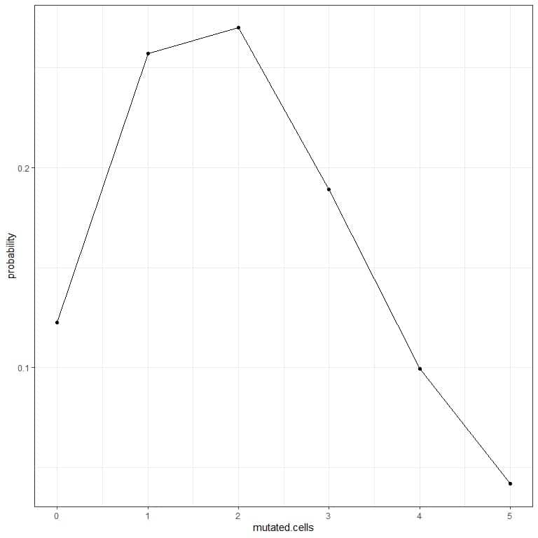
The curve peak is at 2 mutated cells.

For X-rays:

1. Construct a table for the different number of events (mutated cells):

2. Add another column named “average^cells” for the λ^k term. λ is the average events number = 1.4 and k = 0,1,2,3,4,5.

The first value is 1.4^0 = 1.

The second value is 1.4^1 = 1.4.

The third value is 1.4^2 = 1.96, and so on.

3. Add another column named “multiplied average^cells” for the multiplication of average^cells by e^(-λ) = 2.71828^-1.4.

4. Add another column named “probability” by dividing each value of the “multiplied average^cells” by factorial cells.

For 0 cells, the factorial = 1.

For 1 cell, the factorial = 1.

For 2 cells, the factorial = 2X1 = 2.

For 3 cells, the factorial = 3X2X1 = 6, and so on.

5. We can plot the probabilities for the different number of mutated cells, from 0 to 5.

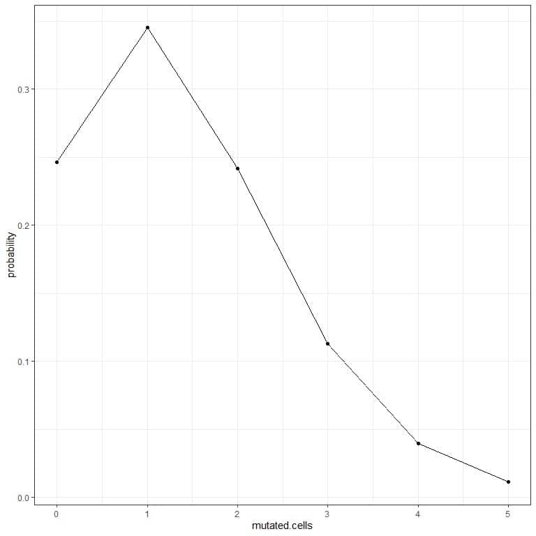The curve peak is at 1 mutated cell.

Practice questions

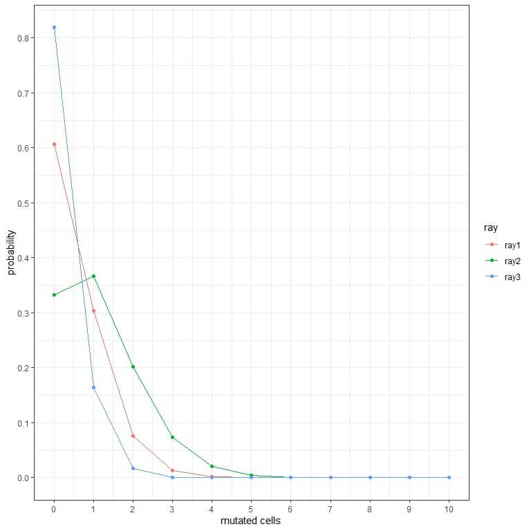
1. In the following plots, we show the probability of the different number of mutated cells when we subject them to different types of rays for a week.

Which are the most dangerous rays?

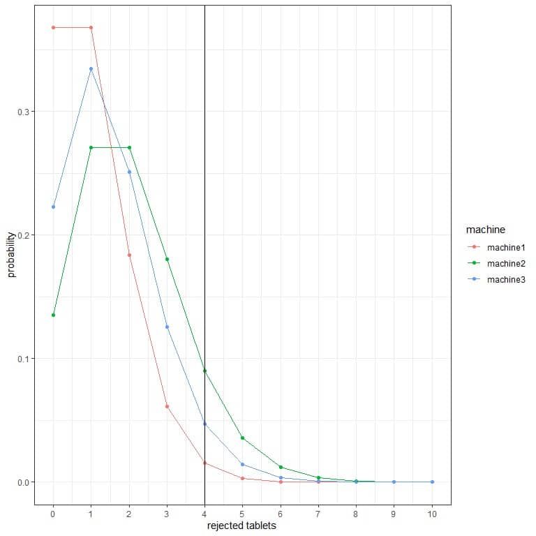
2. In the following plots, we show the probability of the different number of rejected tablets per hour from 3 different machines.

Which is the best machine?

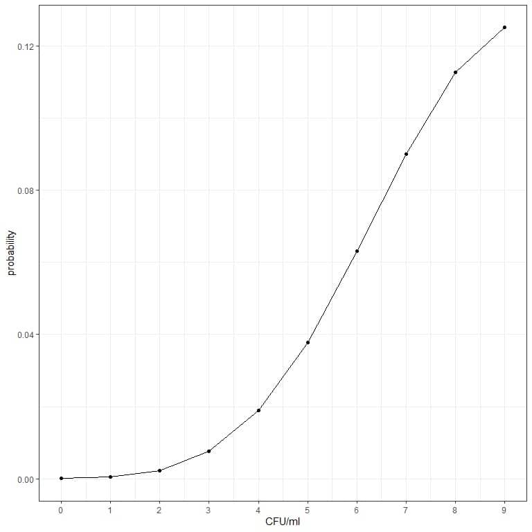
3. The bacterial count average for a certain product is 10 CFU/ml (colony-forming unit/ml). Assuming that the Poisson distribution conditions are met, what is the probability of finding less than 10 CFU/ml?

4. William Feller (1968) modeled Nazi bombing raids on London during World War II using a Poisson distribution. The city was divided into 576 small areas of 1/4 km squared. There were a total of 537 bomb hits, so the average number of hits per area was 537/576 = 0.9323.

How many areas do we expect to be hit by 1 or 2 bombs?

5. The average count of Zanthoxylum panamense trees in 1-hectare square areas in the Barro Colorado Island is 1.34 and follows a Poisson distribution. The total area of this forest is 50 hectares square.

How many hectares do we expect to have no trees of this species?

Answer key

1. The most dangerous rays are ray2 because it has a higher probability for more mutated cells.

For example, the probability of 3 mutated cells in a week for ray2 is nearly 0.1 or 10%, while for ray1 and ray2 is nearly zero.

2. The best machine is machine1 because it has the lowest probability for more rejected tablets.

For example, the probability of 4 rejected tablets in an hour (solid vertical line) in machine2 is higher than in machine3, which is higher than in machine1.

3. The probability of finding less than 10 CFU/ml = probability of 9 CFU/ml + probability of 8 CFU/ml + probability of 7 CFU/ml +………….+ probability of 0 CFU/ml.

• Construct a table for the different number of events (CFU/ml) and add another column named “average^cfu/ml” for the λ^k term. λ is the average bacterial cells/ml = 10 and k = 0,1,2,3,4,5,6,7,8,9.

• Add another column named “multiplied average^cfu/ml” for the multiplication of average^cfu/ml by e^(-λ) = 2.71828^-10.

• Add another column named “probability” by dividing each value of the “multiplied average^cfu/ml” by factorial cfu/ml.

For 0 CFU/ml, the factorial = 1.

For 1 CFU/ml, the factorial = 1.

For 2 CFU/ml, the factorial = 2X1 = 2, and so on.

• We sum the probability column to get the probability of finding less than 10 CFU/ml.

0.00005+ 0.00045+ 0.00227+ 0.00757+ 0.01892+ 0.03783+ 0.06306+ 0.09008+ 0.11260+ 0.12511 = 0.45794 or 45.8%.

• We can plot the probabilities for the different numbers of CFU/ml, from 0 to 9.

4. We calculate the probability of hitting by 1 or 2 bombs:

• Construct a table for the different number of events:

• Add another column named “average^hits” for the λ^k term. λ is the average events number = 0.9323 and k = 1 or 2.

The first value is 0.9323^1 = 0.9323.

The second value is 0.9323^2 = 0.8691833.

• Add another column named “multiplied average^hits” for the multiplication of average^hits by e^(-λ) = 2.71828^-0.9323.

• Add another column named “probability” by dividing each value of the “multiplied average^hits” by factorial hits.

For 1 hit, the factorial = 1.

For 2 hits, the factorial = 2X1 = 2.

The probability of getting hit by 1 bomb = 0.367 or 36.7%.

The probability of getting hit by 2 bombs = 0.17108 or 17.1%.

The probability of hit by 1 or 2 bombs = 0.367+0.17108 = 0.538 or 53.8%.

• We can use these probabilities to calculate the number of areas that are expected to receive these hits.

We multiply each probability by 576 as we have 576 small areas of London.

Out of the total 576 areas of London, we are expecting 211 areas to receive 1 bomb and 98 areas to receive 2 bombs.

5. We calculate the probability of containing zero trees:

• Calculate “average^trees” for the λ^k term. λ is the average events number = 1.34 and k = 0.

λ^k = 1.34^0 = 1.

• Multiply the value you get by e^(-λ) = 2.71828^-1.34.

1 X 2.71828^-1.34 = 0.2618459.

• Calculate the probability by dividing the value of step 2 by factorial trees.

For 0 trees, the factorial = 1.

probability = 0.2618459/1 = 0.2618459.

The probability of seeing no trees of this species = 0.262 or 26.2%.

• We can use this probability to calculate the number of squared hectares expected to contain no trees of this species.

We multiply the probability by 50 as we have 50 squared hectares in this forest.

Expected hectares = 50 X 0.2618459 = 13.0923.

Out of the total 50 squared hectares of this forest, we expect 13 squared hectares to contain no trees of this species.

Previous Lesson | Main Page | Next Lesson