JUMP TO TOPIC
Polar Curves – Definition, Types of Polar Curves, and Examples
 Polar curves give us a better understanding of how we graph equations with a different coordinate system than what we’re used to. In the past, we’ve learned about polar coordinates, so it’s time for us to expand our graphing skills on the polar coordinate system. By the end of our discussion, you’ll see how complex rectangular equations can be graphed easily with the help of common polar curves.
Polar curves are graphs of equations that are defined by polar coordinates. As with regular equations and curves, the polar curve consists of all polar coordinates that satisfy the given equation.
As we have mentioned, we can’t graph polar curves without understanding how the polar coordinate system works. Head over to this link in case you need a quick refresher. In this article, we’ll cover all the fundamental concepts we need to understand polar curves:
- We’ll do a quick refresher on how we plot polar coordinates on polar grids and extend this knowledge to graph curves.
- You’ll also learn how to test a given polar equation’s symmetry and know how to use the result to graph polar curves.
- We’ll provide you a brief discussion on each of the common polar graphs that you’ll be encountering.
Our goal is to cover all the important bases for you and hope that by the end of our discussion, you can work on different problems involving polar curves independently! For now, let’s dive right into the basic components of polar curves.
What is a polar curve?
A polar curve is simply the resulting graph of a polar equation defined by $\boldsymbol{r}$ and $\boldsymbol{\theta}$. We use polar grids or polar planes to plot the polar curve and this graph is defined by all sets of $\boldsymbol{(r, \theta)}$, that satisfy the given polar equation, $\boldsymbol{r = f(\theta)}$.
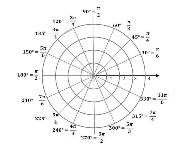
As we have learned in our discussion of polar coordinates, the graph above is a standard example of a polar grid. We call the center the pole and the horizontal axis extending to the right is called the polar axis. The angles outside are the angles that return exact values and this is why they are great references for polar grids as well.
Similar to rectangular coordinate systems, the polar curve of $r = f(\theta)$ will be defined by the polar coordinates satisfying the equation. However, this time, we’re graphing the curve on the polar grid.
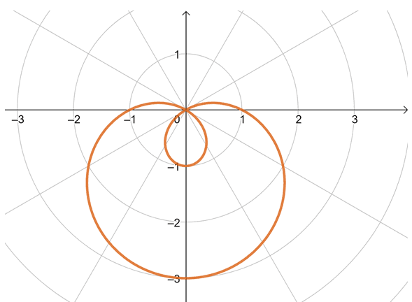
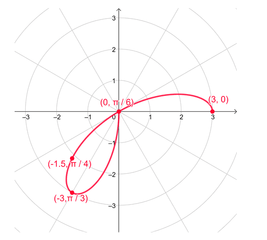
The graph above is an example of a polar curve – this curve, in particular, is defined by the polar equation, $r = 1 – 2\sin \theta$. This means that this curve represents all polar coordinates, $(r, \theta)$, that satisfy the given equation. In the later sections, you’ll learn that this polar curve is in fact a limacon with an inner loop. For now, let’s see how we can use our knowledge of plotting polar coordinates to graph polar curves.
How to graph polar curves?
Polar curves can be graphed by plotting key polar coordinates on the polar grid. This method is similar to graphing rectangular equations – we find input and output values that satisfy the given equation and set up a table of values.
Graphing polar curves by plotting points
We’ll break down the steps of graphing polar curves through this method and remember these pointers when graphing polar curves:
- Construct a partial table of values by assigning different values of $\theta$ from $0$ to $\pi$.
- Since trigonometric functions are periodic, see if you the values for $r$ has repeated.
- Stop when it does and start plotting each polar coordinate (approximate the values of $r$ whenever needed).
- Connect the polar coordinates with a curve and that becomes the polar equation’s graph.
Let’s apply these steps to graph $r = 2 \cos \theta$. We’ll use special angles so that it’ll be easy for us to evaluate each value of $r$. We’ll show you a detailed table of values for this example, but for the next sections, we’ll assume that you can work on the calculations on your own.
| \begin{aligned}\boldsymbol{\theta}\end{aligned} | \begin{aligned}\boldsymbol{r = 2\cos \theta }\end{aligned} | \begin{aligned}\boldsymbol{(r, \theta)}\end{aligned} |
| \begin{aligned} 0\end{aligned} | \begin{aligned} 2 \cos 0 = 2(1) = 2\end{aligned} | \begin{aligned}(4, 0) \end{aligned} |
| \begin{aligned} \dfrac{\pi}{6}\end{aligned} | \begin{aligned} 2 \cos \dfrac{\pi}{6} = 2\left(\dfrac{\sqrt{3}}{2}\right) = \sqrt{3}\end{aligned} | \begin{aligned} \left(\sqrt{3}, \dfrac{\pi}{6} \right) \approx \left(1.73, \dfrac{\pi}{6}\right)\end{aligned} |
| \begin{aligned} \dfrac{\pi}{3}\end{aligned} | \begin{aligned} 2 \cos \dfrac{\pi}{3} = 2\left(\dfrac{1}{2}\right) = 1\end{aligned} | \begin{aligned} \left(1, \dfrac{\pi}{3} \right) \end{aligned} |
| \begin{aligned} \dfrac{\pi}{2}\end{aligned} | \begin{aligned} 2 \cos \dfrac{\pi}{2} = 2\left(0\right) = 0\end{aligned} | \begin{aligned} \left(0, \dfrac{\pi}{2} \right) \end{aligned} |
| \begin{aligned} \dfrac{2\pi}{3}\end{aligned} | \begin{aligned} 2 \cos \dfrac{2\pi}{3} = 2\left(-\dfrac{1}{2}\right) = -1\end{aligned} | \begin{aligned} \left(-1, \dfrac{2\pi}{3} \right) \end{aligned} |
| \begin{aligned} \dfrac{5\pi}{6}\end{aligned} | \begin{aligned} 2 \cos \dfrac{5\pi}{6} = 2\left(-\dfrac{\sqrt{3}}{2}\right) = -\sqrt{3}\end{aligned} | \begin{aligned} \left(-\sqrt{3}, \dfrac{5\pi}{6} \right) \approx \left(-1.73, \dfrac{5\pi}{6}\right) \end{aligned} |
| \begin{aligned}\pi\end{aligned} | \begin{aligned} 2 \cos \pi = 2(1) = 2\end{aligned} | \begin{aligned}(2, \pi) \end{aligned} |
If we continue this table of values, you’ll see that the polar coordinates will repeat. This is why we stop at $\theta = \pi$ and start plotting the polar coordinates we’ve tallied.
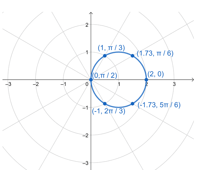
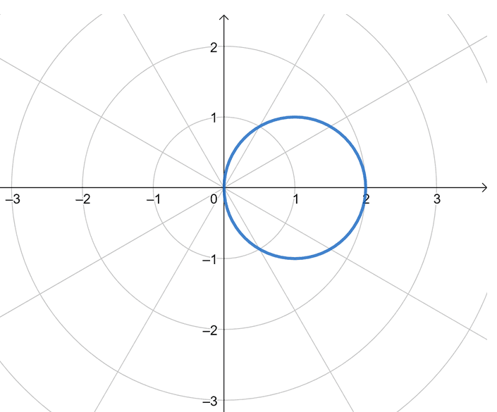
Here’s how the points would appear on one polar grid. We’ve connected the curve as well to finally graph the polar curve representing $r = 2\cos \theta$. To help you see a “neater” polar curve for this equation, we’ll take out the polar coordinates we just used.
Do you notice something about our polar curve? The resulting graph looks like a graph of a circle with a radius of $1$ unit and centered at $(1, 0)$. We can actually confirm this by rewriting $r = 2\cos \theta$ into its rectangular form using this method where we use the rectangular forms of $r$ and $r\cos \theta$.
\begin{aligned}r &= 2\cos \theta\\ r^2 &= 2r\cos \theta\\ x^2 + y^2 &= 2x\\(x^2 – 2x + 1) + y^2 &= 1\\(x -1)^2 + y^2 &= 1 \end{aligned}
In general, polar equations of the form, $\boldsymbol{r= a\cos \theta}$ will be a circle with a radius of $\boldsymbol{\dfrac{a}{2}}$. Don’t worry, we’ve allotted a separate section for these general forms.
For now, let’s see how we can use the symmetry of polar curves to graph them faster.
Understanding the symmetry of polar curves
Polar curves may exhibit symmetry over the polar axis, the line $\boldsymbol{\theta = \dfrac{\pi}{2}}$, or the pole. Once we establish the rules of symmetry for a polar equation, we can evaluate fewer polar coordinates and simply reflect half the curve over whichever it exhibits symmetry on.
These are three symmetry tests you can apply to determine which type of symmetry the polar equation you’re working on exhibits.
Symmetric with Respect Ty}|to the Polar Axis | Symmetric with Respect to the Line $\boldsymbol{\theta = \dfrac{\pi}{2}}$ | Symmetric with Respect to the Pole |
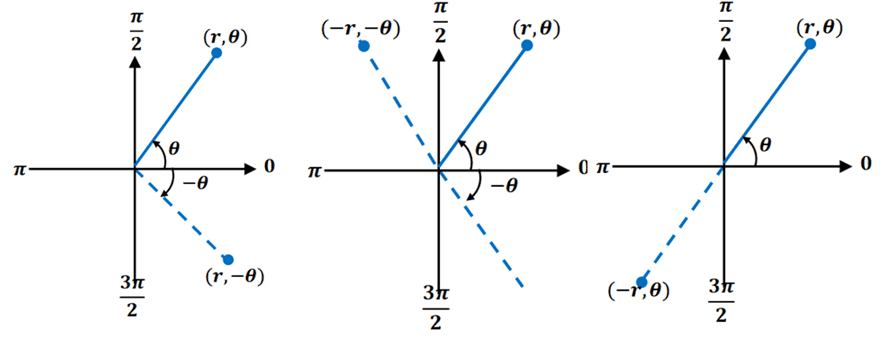
\begin{aligned}(r, \theta) \rightarrow (r, -\theta) \end{aligned} · Simply substitute $\theta$ with its negative equivalent, $-\theta$. · If the resulting expression is identical with our original one, the polar curve is symmetric with respect to the polar axis. | \begin{aligned}(-r, \theta) \rightarrow (-r, -\theta) \end{aligned} · Simply substitute $r$ and $\theta$ with their negative equivalents,$-r$ and $-\theta$. · If the resulting expression is identical with our original one, the polar curve is symmetric with respect to the line $\theta = \dfrac{\pi}{2}$. | \begin{aligned}(r, \theta) \rightarrow (-r, \theta) \end{aligned} · Simply substitute $r$ with its negative equivalent, $-r$. · If the resulting expression is the negative equivalent of our original one, the polar curve is symmetric with respect to the pole. |
If the polar equation passes any of the three symmetry tests, we are guaranteed that its corresponding polar curves will exhibit the same symmetry. Here’s a visual representation of the symmetry that a polar curve may exhibit. We have from left to right: 1) symmetry with respect to the polar axis, 2) symmetry with respect to the line $\boldsymbol{\theta = \dfrac{\theta}{2}}$, and 3) symmetry with respect to the pole.
Here’s an important reminder though: when a polar equation fails the symmetry test, the polar curve may not be or may still exhibit that particular symmetry. But we’ll probably observe that after plotting more polar coordinates. Then, why do we still test the polar equations for symmetry? It’s making sure that we don’t spend more time plotting polar coordinates when we can just reflect parts of the curve over. With fewer polar coordinates that we need to plot, the lesser the chances of any calculations mistake as well!
Graphing polar curves by its symmetry first
Let’s apply what we’ve just learned about symmetries to graph the polar equation, $r = 2\cos 3\theta$. Moving forward, let’s make it a habit to check the polar equation’s symmetry first.
- For the polar axis symmetry: replace $\boldsymbol{\theta}$ with $\boldsymbol{-\theta}$ and see if the resulting expression is still the same.
- For the line $\boldsymbol{\theta = \dfrac{\pi}{2}}$: replace $\boldsymbol{r}$ and $\boldsymbol{\theta}$ with $\boldsymbol{-r}$ and $\boldsymbol{-\theta}$.
- For the pole: replace $\boldsymbol{r}$ with $\boldsymbol{-r}$ and see if the resulting expression is still the same.
| Symmetry Test: Polar Axis | Symmetry Test: Line $\boldsymbol{\theta = \dfrac{\pi}{2}}$ | Symmetry Test: Pole |
| \begin{aligned}r &= 2 \cos(-3\theta)\\&= 3 \cos 3\theta \\&\Rightarrow \textbf{Passed}\end{aligned} | \begin{aligned}(-r) &= 3 \cos(-3\theta)\\-r &= 3 \cos 3\theta \\r &= -3\cos 3\theta \\&\Rightarrow \textbf{Failed}\end{aligned} | \begin{aligned}(-r) &= 3 \cos(3\theta)\\-r &= 3 \cos 3\theta \\r &= -3\cos 3\theta \\&\Rightarrow \textbf{Failed}\end{aligned} |
From the results, we can conclude that the polar equation, $r = 2\cos 3\theta$, is symmetric with respect to the polar axis. Let’s evaluate some values of $\theta$ within $\left[0, \dfrac{\pi}{2}\right]$.
| $\boldsymbol{\theta}$ | $0$ | $\dfrac{\pi}{6}$ | $\dfrac{\pi}{4}$ | $\dfrac{\pi}{3}$ | $\dfrac{\pi}{2}$ |
| $\boldsymbol{r}$ | $3$ | $0$ | $-2.1$ | $-3$ | $0$ |
Plot these polar coordinates then connect these points with a curve as shown below.
Since we’ve confirmed that $r = 3\cos 3\theta$ is symmetric with respect to the polar axis, let’s graph the remaining half of the curve by reflecting what we have over the polar axis.
Hence, we have the polar curve shown above- we call this polar curve a rose. This shows that the polar equation, $r = 3\cos 3\theta$, is a rose with three petals and is symmetric with respect to the polar axis. In fact, all polar equations of the form, $\boldsymbol{r = a \cos n\theta}$, will return a rose with $\boldsymbol{n}$ petals.
Types of polar graphs
We’ve already shown you examples of polar curves: a circle, a limacon, and a rose, to be exact. In this section, we’ll summarize all common polar graphs you’ll encounter along with their general forms.
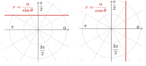
Lines: If the polar equation has a general form of $r = \dfrac{a}{\sin \theta}$ or $r = \dfrac{a}{\cos \theta}$, where $a \neq 0$, its curve will be a horizontal line or a vertical line, respectively. The line passes through either $(0, a)$ or $(a, 0)$.
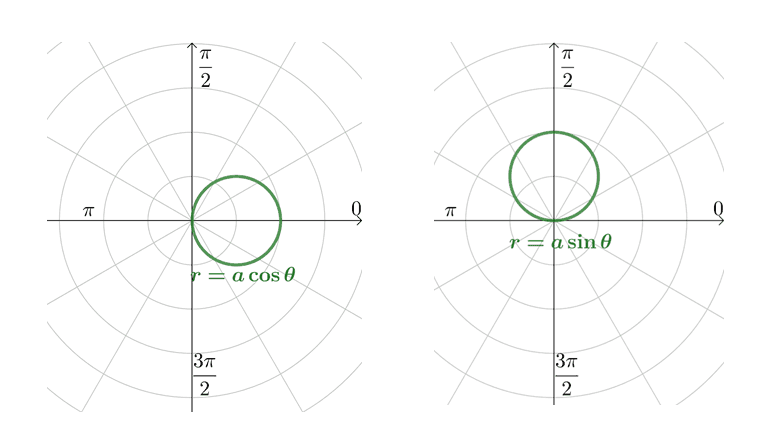
Circles: If the polar equation has a general form of $r = a\cos \theta$ or $r = a\sin \theta$, where $a > 0$, its curve will be a circle with a radius of $\dfrac{a}{2}$.
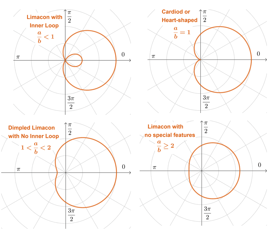
Limacons: If the polar equation has a general form of $r = a \pm b\cos \theta$ or $r = a \pm b\sin \theta$, where $a,b > 0$, its curve will be a curve called the limacon (it’s French for snail). You’ll encounter four variations of limacons and their shape depends on the value of $\dfrac{a}{b}$.
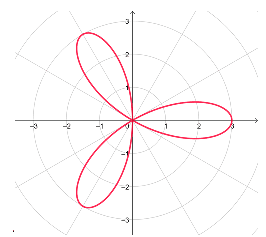
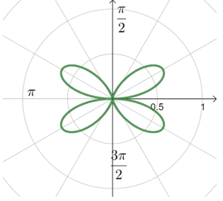
Rose: If the polar equation has a general form of $r = a \cos n\theta$ or $r = a\sin n\theta$, where $a \neq 0$, its graph will be a polar curve called the rose. We call each segment of the rose petals and the number of petals will depend on whether $n$ is even or odd.
- If $n$ is even, the polar curve (rose) will show $2n$ petals.
- If $n$ is odd, the polar curve (rose) will show $n$ petals.
Here are examples of a rose with an odd number of petals and a rose with an even number of petals.
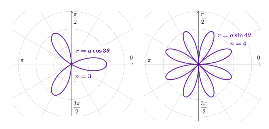
For $r = a\cos 3\theta$, we expect the rose to have $n = 3$ petals while for $r = a\sin 4\theta$, we are expecting $2n = 8$ petals from the rose.
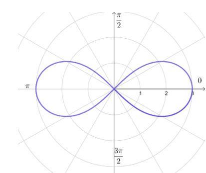
Lemniscate: If the polar equation has a general form of $r^2 = a^2 \cos 2\theta$ or $r = a^2 \sin 2\theta$, where $a \neq 0$, its curve will be called a lemniscate.
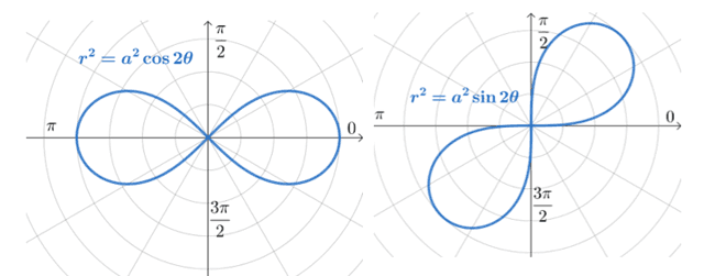
The length of each “propeller” is $a$. For the polar curve of $r^2 =a^2\cos 2\theta$, the graph is symmetric with respect to the polar axis, the pole, and the line, $\theta = \dfrac{pi}{2}$. Meanwhile, $e^2 =a^2\sin 2\theta$ is symmetric with respect to the pole.
These are five types of polar graphs that you’ll commonly encounter. Familiarizing yourself with their general forms and properties will definitely help you save time when graphing different polar equations. We’ve prepared more sample problems for you to work on and test your understanding of polar graphs. When you’re ready, head over to the next section!
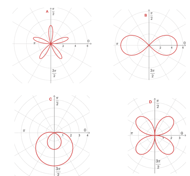
Example 1
\begin{aligned}r =2- 4\cos\theta &, r= 1+ \sin \theta \\r = 4\cos 6\theta&, r =3\cos\theta \end{aligned}
The polar curves of these four polar equations are as shown below. Match the polar equations with their corresponding polar curve.
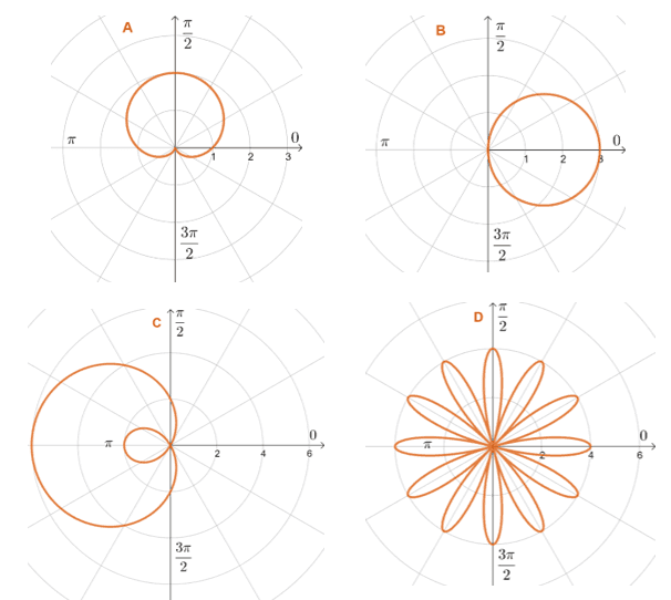
Solution
There is no need for us to graph each polar equation individually. That’s the benefit of knowing the common polar graphs’ general forms. We’ll identify the polar equation’s general form then use that to determine its polar curve’s shape.
Starting with $\boldsymbol{r =2- 4\cos\theta}$, we can see that its general form is $r = a – b \cos \theta$.
- This general form would return a limacon. Now, let’s take a look at $\dfrac{a}{b} = \dfrac{1}{2}$.
- Since this is less than $1$, the limacon will have an inner loop with a length of $1$ unit.
- This means that $r = 2 – 4\cos \theta$ will have a limacon with an inner loop making C the correct polar curve representing it.
We’ll apply a similar thought process for the rest of the polar equations and we’ve summarized the results in one table.
| Polar Equation | General Form | Polar Curve |
| \begin{aligned} r= 2- 4\cos \theta\end{aligned} | \begin{aligned}a + b \cos \theta &\Rightarrow \text{Limacon}\\ \dfrac{a}{b} = \dfrac{1}{2} &\Rightarrow \text{with Inner Loop} \end{aligned} | \begin{aligned}\textbf{C}\end{aligned} |
| \begin{aligned} r= 1+ \sin \theta\end{aligned} | \begin{aligned}a + b \sin \theta &\Rightarrow \text{Limacon}\\ \dfrac{a}{b} = 1 &\Rightarrow \text{Dimpled Limacon} \end{aligned} | \begin{aligned}\textbf{A}\end{aligned} |
| \begin{aligned} r =4\cos 6\theta\end{aligned} | \begin{aligned} a\cos n\theta &\Rightarrow \text{Rose}\\ n = 6 &\Rightarrow \text{12 Petals} \end{aligned} | \begin{aligned}\textbf{D}\end{aligned} |
| \begin{aligned} r = 3\cos \theta\end{aligned} | \begin{aligned} a\cos \theta &\Rightarrow \text{Circle}\\ a = 3 &\Rightarrow \text{Radius of 1.5} \end{aligned} | \begin{aligned}\textbf{B}\end{aligned} |
Example 2
Test whether $r = 4 \cos \theta$ is symmetric with respect to the polar axis, the line $\theta = \dfrac{\theta}{2}$, or the pole.
Solution
When testing for symmetry with respect to the pole, we replace $\theta$ with $-\theta$ and see if it still returns the original polar equation.
\begin{aligned}r &= 4 \cos (-\theta)\\&= 4\cos \theta\\ &\Rightarrow \textbf{Passed} \end{aligned}
This means that $r = 4\cos\theta $ is symmetric with respect to the polar axis.
Now, let’s test $r = 4\cos \theta$ for symmetry with respect to the line $\theta = \dfrac{\pi}{2}$ by replacing both $r$ and $\theta$ with $-r$ and $-\theta$.
\begin{aligned}(-r) &= 4 \cos (-\theta)\\ -r &= 4\cos \theta\\r &= -4\cos \theta &\Rightarrow \textbf{Failed} \end{aligned}
Using the symmetry tests, we can’t guarantee that the polar equation is symmetric with respect to the pole. Keep in mind that failing the particular symmetry test is inconclusive. We’ll now work on the third symmetry test for the pole – replace $r$ with $-r$.
\begin{aligned}(-r) &= 4 \cos \theta\\ r &= -4\cos \theta &\Rightarrow \textbf{Failed} \end{aligned}
The polar equation, $r =4\cos \theta$ didn’t pass the third symmetry test. This means that we can only guarantee that the polar equation is symmetric with respect to the polar axis.
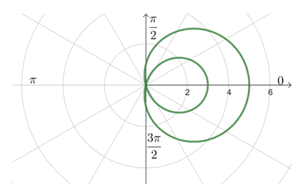
Example 3
Test $r^2 = 9\cos 2\theta$ for symmetry then graph its polar curve.
Solution
Use the three symmetry tests to see if $r^2 =9\cos2\theta$ is symmetric with respect to either the polar axis, the line $\theta=\dfrac{\pi}{2}$, or the pole.
| Symmetry Test: Polar Axis | Symmetry Test: Line $\boldsymbol{\theta = \dfrac{\pi}{2}}$ | Symmetry Test: Pole |
| \begin{aligned}r^2 &= 9 \cos 2(-\theta)\\&= 9 \cos 2\theta \\&\Rightarrow \textbf{Passed}\end{aligned} | \begin{aligned}(-r)^2&= 9 \cos 2(-\theta)\\r^2 &= 9\cos 2\theta \\&\Rightarrow \textbf{Passed}\end{aligned} | \begin{aligned}(-r)^2 &= 9 \cos 2(-\theta)\\r^2 &= 9\cos 2\theta \\&\Rightarrow \textbf{Passed}\end{aligned} |
The polar equation passed all three symmetry tests and this makes sense since its general form is $r^2 = a^2\cos \theta$. This is a lemniscate that is symmetric with respect to all three: the polar axis, pole, and the line $\theta=\dfrac{\pi}{2}$.
This also means that we’re expecting the graph to be a lemniscate with each “wing” having a length of $3$ units. For now, let’s plot some polar coordinates to graph half of its curve (and to get a more accurate shape).
| $\boldsymbol{\theta}$ | $0$ | $\dfrac{\pi}{6}$ | $\dfrac{\pi}{4}$ |
| $\boldsymbol{r}$ | $\pm3$ | $\pm2.1$ | $0$ |
Plot the polar coordinates: $(3,0)$, $\left(2.1, \dfrac{\pi}{6}\right)$,and $\left(0, \dfrac{\pi}{4}\right)$.
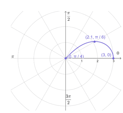
Reflect the curve over the polar axis then reflect it along the line $\theta = \dfrac{\pi}{2}$. This will cover all portions of the lemniscate that we need to graph.
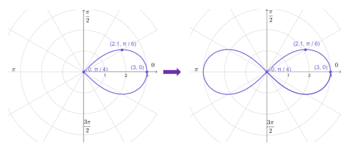
Hence, we have the graph of $r^2 = 9 \cos 2\theta$ – a lemniscate that is symmetric with respect to the pole, polar axis, and the line $\theta =\dfrac{\pi}{2}$.
This example highlights the importance of understanding the symmetry test and the general forms of the polar curves. Knowing them by heart will definitely save you time and avoid mistakes in the future!
Practice Questions
1. \begin{aligned}r =3\sin 5\theta &, r= 3\sin 2\theta \\r = 1 – 3\sin \theta&, r^2 = 25\sin 2\theta \end{aligned}
The polar curves of these four polar equations are as shown below. Match the polar equations with their corresponding polar curve.
2. Test whether $r^2 = 16\sin 2\theta$ is symmetric with respect to the polar axis, the line $\theta = \dfrac{\theta}{2}$, or the pole.
3. Test the following polar equations for symmetry then graph its polar curve.
a. $r = 1 – 4\sin \theta$
b. $r = \dfrac{4}{1 – \sin \theta}$
c. $r =\cos^2\theta\sin\theta$
Answer Key
1. $\begin{aligned}r &=3\sin 5\theta \Rightarrow\textbf{A} \\r &= 3\sin 2\theta\Rightarrow\textbf{D} \\r &= 1 – 3\sin \theta \Rightarrow\textbf{C}\\r^2 &= 25\sin 2\theta\Rightarrow\textbf{B} \end{aligned}$
2. $r^2 = 16\sin 2\theta$ is symmetric with respect to the pole.
3.
a. Symmetric with respect to the polar axis.
b. Can’t guarantee symmetry through the pole, polar axis, and the line $\theta = \dfrac{\pi}{2}$.
c. Symmetric with respect to the pole.
Images/mathematical drawings are created with GeoGebra.