The Population Mean – Explanation & Examples

The definition of the population mean is:

“The population mean is the mean or average found in a population.”

In this topic, we will discuss the population mean from the following aspects:

• What is the population mean?
• How to find the population mean?
• The population mean formula.
• The role of the population mean.
• Practice questions.
• Answer key.

What is the population mean?

The population mean is the mean value of a numerical characteristic of the population. The population is the whole group of items we want to study. These items can be individuals, things, animals, plants, etc.

For example, the whole individuals living in the U.S., the whole chairs produced from a certain factory, the whole tigers living in rain forests in Indonesia, and the whole orange trees in Egypt.

These different populations’ numerical characteristics can be weights for individuals, leg lengths for chairs, tail lengths for tigers, and the heights for orange trees.

However, collecting information from the population may not be possible in many cases due to the great resources it needs.

For example, if we want to study the heights of American males. We can survey every American male and get his height. This is population data.

Alternatively, we can select 200 American males and measure their heights. This is sample data.

If we calculate the mean of the population data, its symbol is the Greek letter μ and pronounced “mu.”

How to find the population mean?

We have two cases:

1. We have population data and so calculate the population mean from it.
2. We have sample data and use the sample mean to construct an interval that most likely contains the population mean.

– Examples of population data

– Example 1

The following is the murder rate (per 100,000 population) for the 50 states of the U.S. in 1976. What is the mean of the murder rate?

We have information about all states of the U.S. so this is population data.

Note

This dataset may be considered as a sample or as a population.

It is a sample if we want to study the murder rate of the U.S. states in the 1970s, or it is a population if data is from 1970-1980 because this is a 1-year sample from these 10 years.

It is a population for the murder rate of U.S. states in 1976.

1. Add up all of the numbers:

15.1+ 11.3+ 7.8+ 10.1+ 10.3+ 6.8+ 3.1+ 6.2+ 10.7+ 13.9+ 6.2+ 5.3+ 10.3+ 7.1+ 2.3+ 4.5+ 10.6+ 13.2+ 2.7+ 8.5+ 3.3+ 11.1+ 2.3+ 12.5+ 9.3+ 5.0+ 2.9+ 11.5+ 3.3+ 5.2+ 9.7+ 10.9+ 11.1+ 1.4+ 7.4+ 6.4+ 4.2+ 6.1+ 2.4+ 11.6+ 1.7+ 11.0+ 12.2+ 4.5+ 5.5+ 9.5+ 4.3+ 6.7+ 3.0+ 6.9 = 368.9.

2. Count the numbers of items in your population. In this population, there are 50 items or 50 states.

3. Divide the number you found in Step 1 by the number you found in Step 2.

The population mean = 368.9/50 = 7.378.

Note that the population mean has the same unit as the original data. So 7.378 is the mean murder rate per 100,000 population.

– Example 2

The following are the weights (in grams) for 71 chickens on a certain farm. What is the mean?

We have the weights of all chickens on the farm, so this is population data.

1. Add up all of the numbers:

179+ 160+ 136+ 227+ 217+ 168+ 108+ 124+ 143+ 140+ 309+ 229+ 181+ 141+ 260+ 203+ 148+ 169+ 213+ 257+ 244+ 271+ 243+ 230+ 248+ 327+ 329+ 250+ 193+ 271+ 316+ 267+ 199+ 171+ 158+ 248+ 423+ 340+ 392+ 339+ 341+ 226+ 320+ 295+ 334+ 322+ 297+ 318+ 325+ 257+ 303+ 315+ 380+ 153+ 263+ 242+ 206+ 344+ 258+ 368+ 390+ 379+ 260+ 404+ 318+ 352+ 359+ 216+ 222+ 283+ 332 = 18553.

2. Count the numbers of items in your population. In this population, there are 71 items or chickens.
3. Divide the number you found in Step 1 by the number you found in Step 2.

The population mean = 18553/71 = 261.3 grams.

– Example 3

The following is the trunk circumference (in mm) for 35 orange trees on a certain farm. What is the mean?

We have the trunk circumferences of all trees on the farm, so this is population data.

1. Add up all of the numbers:

30+ 58+ 87+ 115+ 120+ 142+ 145+ 33+ 69+ 111+ 156+ 172+ 203+ 203+ 30+ 51+ 75+ 108+ 115+ 139+ 140+ 32+ 62+ 112+ 167+ 179+ 209+ 214+ 30+ 49+ 81+ 125+ 142+ 174+ 177 = 4055.

2. Count the numbers of items in your population. In this population, there are 35 items or trees.

3. Divide the number you found in Step 1 by the number you found in Step 2.

The population mean = 4055/35 = 115.8571 mm.

– Examples of sample data

For samples with a size greater than 30, the interval that, most likely, contains the population mean is calculated by:

¯x±1.96Xs/√n

Where:

¯x is the calculated sample mean.

s is the standard deviation of the sample. It is a measure of the data spread.

n is the sample size.

This interval (called 95% confidence interval) gives us a range of possible values for the unknown population mean from which the sample was taken.

– Example 4

The following is the age (in years) of 50 randomly selected individuals from a certain population. If you know that this sample’s standard deviation is 18.65, construct a 95% confidence interval for the true population mean.

89 61 74 85 46 60 41 18 37 30 44 37 51 53 74 38 56 48 52 62 33 56 38 30 43 32 74 27 49 53 40 27 42 60 88 22 59 43 69 75 28 47 35 62 65 31 22 31 26 83.

1. Add up all of the numbers in your sample:

89+ 61+ 74+ 85+ 46+ 60+ 41+ 18+ 37+ 30+ 44+ 37+ 51+ 53+ 74+ 38+ 56+ 48+ 52+ 62+ 33+ 56+ 38+ 30+ 43+ 32+ 74+ 27+ 49+ 53+ 40+ 27+ 42+ 60+ 88+ 22+ 59+ 43+ 69+ 75+ 28+ 47+ 35+ 62+ 65+ 31+ 22+ 31+ 26+ 83 = 2446.

2. Count the numbers of items in your sample. In this sample, there are 50 items or persons.

3. Divide the number you found in Step 1 by the number you found in Step 2.

The sample mean = 2446/50 = 48.92 years.

4. The 95% confidence interval is:

¯x±1.96Xs/√n

¯x-1.96Xs/√n to ¯x+1.96Xs/√n

48.92-1.96X18.65/√50 to 48.92+1.96X18.65/√50 or 43.75 to 54.1.

It means that the true population mean age can be as small as 43.75 years and as large as 54.1 years.

Owing to the presence of the √n term in the formula for an interval calculation, the sample size affects the interval width. Larger sample sizes lead to smaller interval widths (or a more precise estimate of the population mean).

Suppose that you have a 100 sample size and you obtain the same sample mean and standard deviation; the 95% confidence interval will be:

48.92-1.96X18.65/√100 to 48.92+1.96X18.65/√100 or 45.26 to 52.6.

Suppose that you have a 500 sample size and you obtain the same sample mean and standard deviation; the 95% confidence interval will be:

48.92-1.96X18.65/√500 to 48.92+1.96X18.65/√500 or 47.29 to 50.55.

With increasing the sample size, you have more values about the true population mean.

We can see that in the following figure.

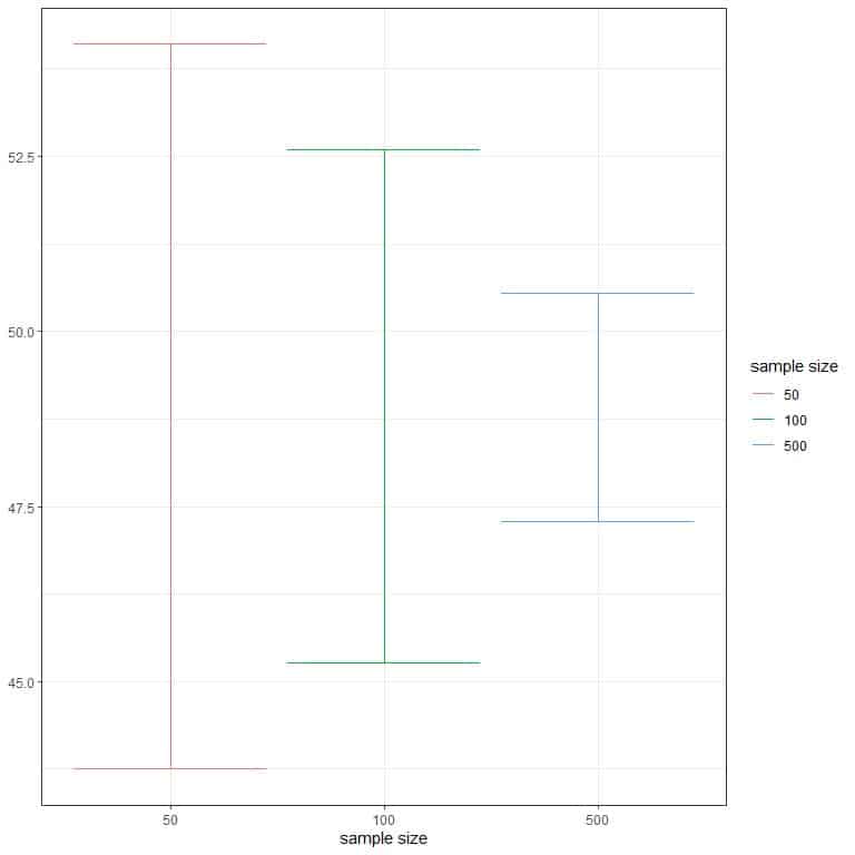
Increasing the sample size has led to a narrower confidence interval.

– Example 5

Plotting the confidence intervals for different random samples

We have a population data of more than 20,000 individuals. We know that the true population mean for the age of these 20,000 individuals is 47.18 years.

Using a computer program, we will take 50 random samples from this population, each of size 35, and calculate the mean’s confidence interval for each sample.

Add another column to the table to indicate if the interval covers the true population mean.

The interval will not cover the population mean if the lower limit is higher than the population mean or the upper limit is lower than the population mean.

Then, we will plot these confidence intervals to see how they cover the true population mean.

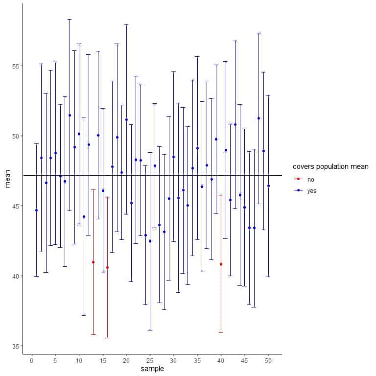
The horizontal black line represents the true population mean.

The blue or red dots represent the mean calculated from each random sample.

The error bars represent the confidence interval calculated from each sample.

We see only 3 samples create a confidence interval that does not cover the population mean and accounting for 3/50 = 0.06 or 6%. Hence, it is very unlikely that the created confidence interval does not cover the population mean.

In research, we take only 1 sample and construct a 95% confidence interval from it.
We do not know if our sample yields an interval containing the population value or one of the bad samples that yield an interval not containing the population value.

However, the constructed 95% confidence interval works 95% of the time. We can assume that the constructed interval has the population value.

Population mean formula

The population mean formula is:

μ=1/N∑X

Where μ is the population mean.

N is the population size.

∑X means the sum of every element in our population.

We used this formula in the above examples, where we summed the population data and divided it by the population size (or multiplied by 1/N).

The role of the population mean

The population mean gives us a measure of the center or central tendency of the population data.

This is useful when comparing different populations to each other.

– Example 1

The following table is the mean age for certain male and female populations.

We see that the mean age is nearly similar for males and females.

It means that the ages for males and females are similar in their distributions. We can see that from plotting the ages for both populations as histograms.

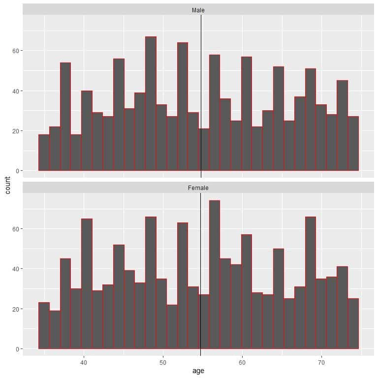The black vertical line represents the mean for each group.

We can also plot the data as a dot plot to see individual values.

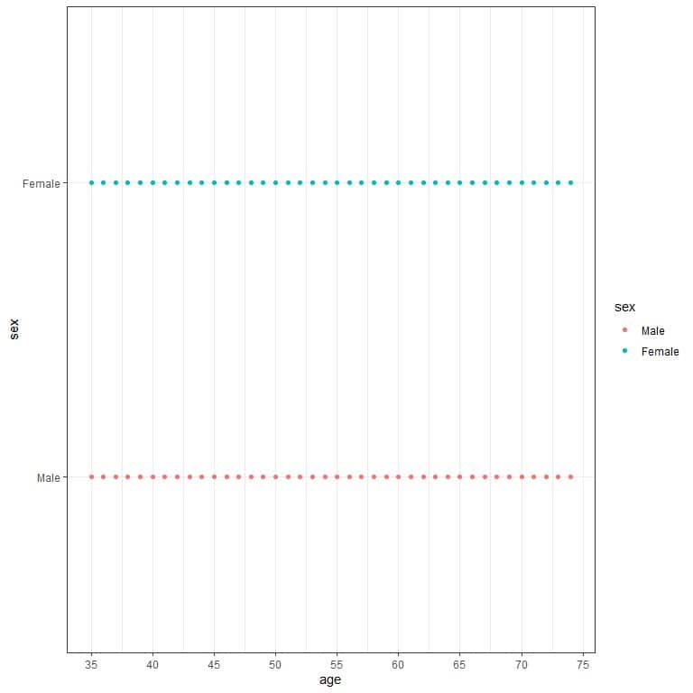
We see the same range for male and female ages.

– Example 2

The following table is the mean height for certain male and female populations.

We see that the mean height for males is higher than the mean height for females.

Without looking at the data, this male population’s heights are longer than the heights of this female population on average.

We can see that from plotting the heights for the 2 populations as histograms.

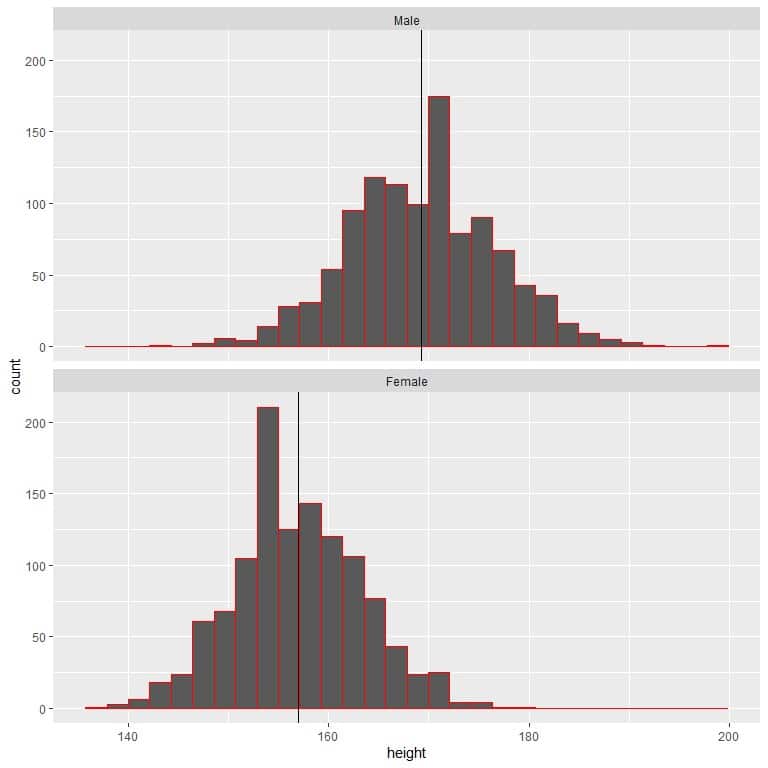
The black vertical line represents the mean for each group.

We can also plot the data as a dot plot to see individual values.

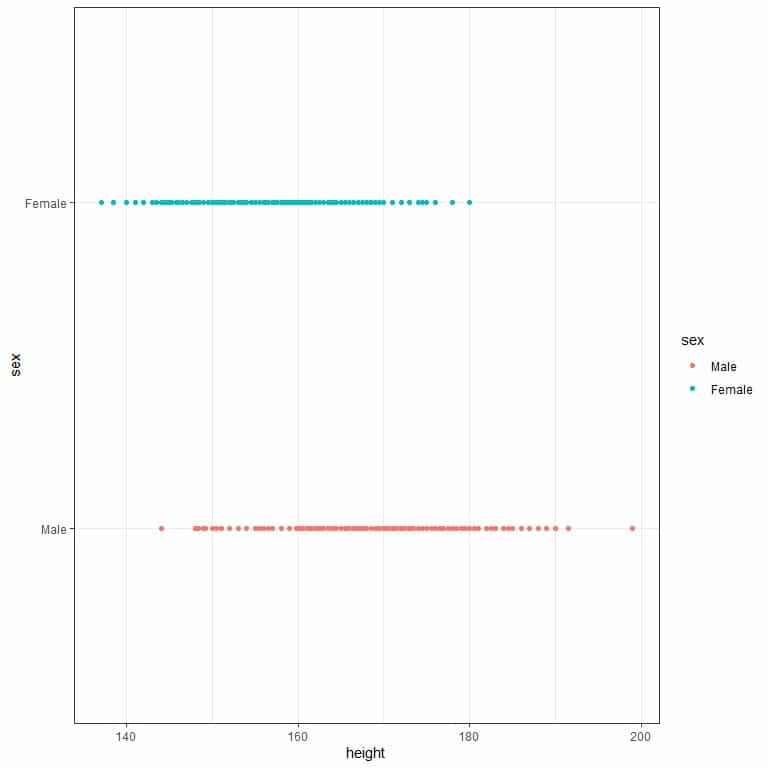
We see that males’ height tends to be longer than females’ height.

But what about the sample means?

The sample means also give information about the population data center from which the sample was collected.

However, we have to calculate the 95% confidence interval for each sample mean due to sampling error. Suppose the confidence intervals do not overlap for the two samples. In that case, we can deduce that the two populations (from which the two samples were taken) are significantly different from each other.

– Example 3

The following table is the birth weight of neonates (in grams) for a random sample of 35 smoking and 35 never-smoking mothers.

The mean birth weight for the smoking mothers = 2899 grams, while the mean for never-smoking mothers = 2946 grams.

The standard deviation for smoking mothers’ weight = 576.72 grams, while the standard deviation for never-smoking mothers = 783.22 grams.

While the sample mean for never-smoking mothers is larger than that for smoking mothers, one may argue that this difference is due to sampling error and not due to the true difference between the population of smoking and never-smoking mothers.

To overcome that, we construct a 95% confidence interval for each mean:

The 95% confidence interval for smoking mothers is:

2899-1.96X576.72/√35 to 2899+1.96X576.72/√35 or 2707.9 to 3090.1.

The 95% confidence interval for never smoking mothers is:

2946-1.96X783.22/√35 to 2946+1.96X783.22/√35 or 2686.5 to 3205.5.

The two confidence intervals overlap, so we conclude that there is no difference in the mean neonate birth weight for smoking and never smoking mothers.

Practice questions

1. The following is the income per capita for the 50 states of the U.S. in 1974. What is the mean income per capita?

2. The following is the miles/U.S. gallon (mpg) for 32 car models in a certain car showroom (in the 1970s). What is the mean of this population?

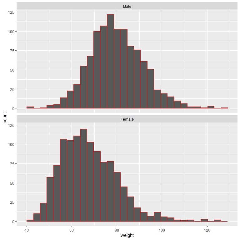
3. The following two histograms are for the weights of certain male and female populations. Can you deduce which population has a higher mean weight?

3. The following table is for the mean wind speed for different classes of storm populations.

And the following dot plot is for the data values (wind speed) of these classes.

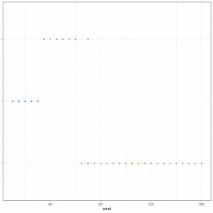
We have many data values, but as they are equal in value, the points are superimposed.

Which points correspond to which mean?

5. You have two samples of diamonds. One sample is 38 ideal-cut diamonds, and the mean weight is 0.703 grams, and the standard deviation is 0.4. The second sample is 45 fair-cut diamonds, and the mean weight is 1.25 grams, and the standard deviation is 0.5.

Assuming that the two samples are randomly selected from a certain batch of diamonds in a certain factory. Is there a difference in the mean weight between the ideal and fair-cut diamonds in this batch?

Answer key

1. This is population data so we can calculate the population mean directly:

• Sum of all numbers = 221790.
• Count the numbers of items in.your population. In this population, there are 50 items or states.
• Divide the first number by the second number.

The population mean = 221790/50 = 4435.8.

2. This is population data so we can calculate the population mean directly:

• Sum of all numbers = 642.9.
• In this population, there are 32 items or models.
• Divide the first number by the second number.

The population mean = 642.9/32 = 20.09 mpg.

3. We see that males’ weight tends to be heavier than females’ weight (more shifted to the right), so males’ mean weight will be larger than the mean weight for females.

4. Red points correspond to hurricane class, blue points to a tropical storm, and green points to a tropical depression.

It is because each group of dots’ center corresponds to the calculated mean value in the table.

5. We construct a 95% confidence interval for each mean:

The 95% confidence interval for the ideal-cut diamonds is:

0.703-1.96X0.4/√38 to 0.703+1.96X0.4/√38 or 0.58 to 0.83.

The 95% confidence interval for fair-cut diamonds is:

1.25-1.96X0.5/√45 to 1.25+1.96X0.5/√45 or 1.10 to 1.396.

The two confidence intervals do not overlap, so we conclude that fair-cut diamonds have a significantly heavier weight than ideal-cut diamonds in this batch.

Previous Lesson | Main Page | Next Lesson