The Random Variable – Explanation & Examples

The definition of a random variable is:

“The random variable is a set of numerical values from a random process.”

In this topic, we will discuss the random variable from the following aspects:

• What is a random variable?
• Discrete random variable.
• Continuous random variable.
• Practice questions.
• Answer key.

What is a random variable?

The random variable is a set of possible numerical values or outcomes from a random process.

A random process is an event that has a random outcome. Random process means that you can not exactly predict its outcome.

For example, throwing a die, tossing a coin, or choosing a card.

Random variables give numbers to outcomes of random events.

– Example 1

If we are tossing a coin (random event) and the outcome can be a head or a tail (random variable). There are only two possible outcomes.

You can give a number to every outcome. Your random variable could be equal to 1 if you get a head and 0 if you get a tail.

We use a capital letter, like X, to denote a random variable.

We denote that as X = {0,1}, meaning that the random variable X can randomly take a value of 0 or 1 (or tail and head).

Note: we can assign any other two numbers to heads and tails. It is our choice.

So:

• We have a random process (such as tossing a coin).
• We give a number to each outcome from this random process.
• The set of these numbers is a random variable.

– Example 2

If we are throwing a die (random process), the score we get on the top face is the random variable. There are only six possible outcomes (1,2,3,4,5,or 6).

You can give the same number to the score you get

Your random variable equals 1 if you get 1.

Your random variable equals 2 if you get 2.

Your random variable equals 3 if you get 3.

Your random variable equals 4 if you get 4.

Your random variable equals 5 if you get 5.

Your random variable equals 6 if you get 6.

We denote that as X = {1,2,3,4,5,6}, meaning that the random variable X can take a value of 1,2,3,4,5, or 6 randomly.

– Example 3

Suppose we are selecting an individual from a population and measuring his height (random event). The person’s height is the random variable.

There are many possible heights that you can get.

Examples 1 and 2 are examples of discrete random variables, while example 3 is an example of a continuous random variable.

The probability distribution for a random variable describes how the probabilities are distributed over the random variable’s different values.

For the discrete random variable, the probability distribution is called the probability mass function.

For the continuous random variable, the probability distribution is called the probability density function.

In any probability distribution, the probabilities must be >= 0 and sum to 1.

Discrete random variable

Discrete random variables take a countable number of integer values and cannot take decimal values. Discrete random variables are usually counts.

Examples of discrete random variables:

• The score you get when throwing a die.
• The number of defective piston rings in a box of ten.

– Example 1

You are tossing a coin. The random variable equals 1 if you get a head and 0 if you get a tail.

You tossed the coin 100 times and get the following results:

0 1 0 1 1 0 1 1 1 0 1 0 1 1 0 1 0 0 0 1 1 1 1 1 1 1 1 1 0 0 1 1 1 1 0 0 1 0 0 0 0 0 0 0 0 0 0 0 0 1 0 0 1 0 1 0 0 1 1 0 1 0 0 0 1 0 1 1 1 0 1 1 1 0 0 0 0 1 0 0 0 1 0 1 0 0 1 1 1 0 0 1 0 1 0 0 1 0 0 1.

You get 53 zeros and 47 ones. You can use that data to estimate the probability mass function (or the probability distribution) for tossing this coin.

The probability for heads or ones = 47/100 = 0.47.

The probability for tails or zeros = 53/100 = 0.53.

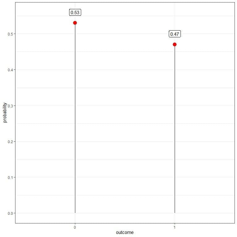
All probabilities are >= 0 and sum to 1.

It is a likely fair coin where the probability of heads nearly equals the probability of tails = 0.5.

We do not get exactly 50 heads and 50 tails due to randomness in the process, but we get a good approximation to the probability of the fair coin = 0.5.

What if we have an unfair coin?

We tossed this coin and get the following results:

1 1 1 0 0 1 1 0 1 1 0 1 1 1 1 0 1 1 1 0 0 1 1 0 1 1 1 1 1 1 0 0 1 1 1 1 1 1 1 1 1 1 1 1 1 1 1 1 1 0 1 1 1 1 1 1 1 1 0 1 1 1 1 1 0 1 0 0 1 1 1 1 1 1 1 1 1 1 1 1 1 1 1 1 1 1 0 0 0 1 1 1 1 1 1 1 1 1 1 1.

You get 18 zeros and 82 ones. We can use that data to estimate the probability mass function for tossing this coin.

The probability for heads or ones = 82/100 = 0.82.

The probability for tails or zeros = 18/100 = 0.18.

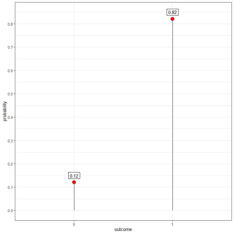
It is a likely unfair coin where heads’ probability is quite larger than the probability of tails.

– Example 2

You are throwing a die. The random variable can be 1, 2, 3, 4, 5, or 6 randomly.

You threw the die 100 times and get the following results:

3 6 4 1 1 2 5 1 5 4 1 4 6 5 2 1 3 2 3 1 1 6 5 1 5 6 5 5 3 2 1 1 6 6 2 4 6 3 3 3 2 4 4 4 2 2 3 4 3 1 2 4 6 2 5 3 2 6 1 4 5 2 4 3 6 4 6 6 6 4 6 5 6 2 4 3 4 5 4 2 3 6 4 6 2 4 1 1 1 3 2 5 4 5 3 3 6 2 4 5.

In a table form:

You can use that data to estimate the probability mass function for throwing this die.

The probability for ones = 15/100 = 0.15.

The probability for twos = 17/100 = 0.17, and so on.

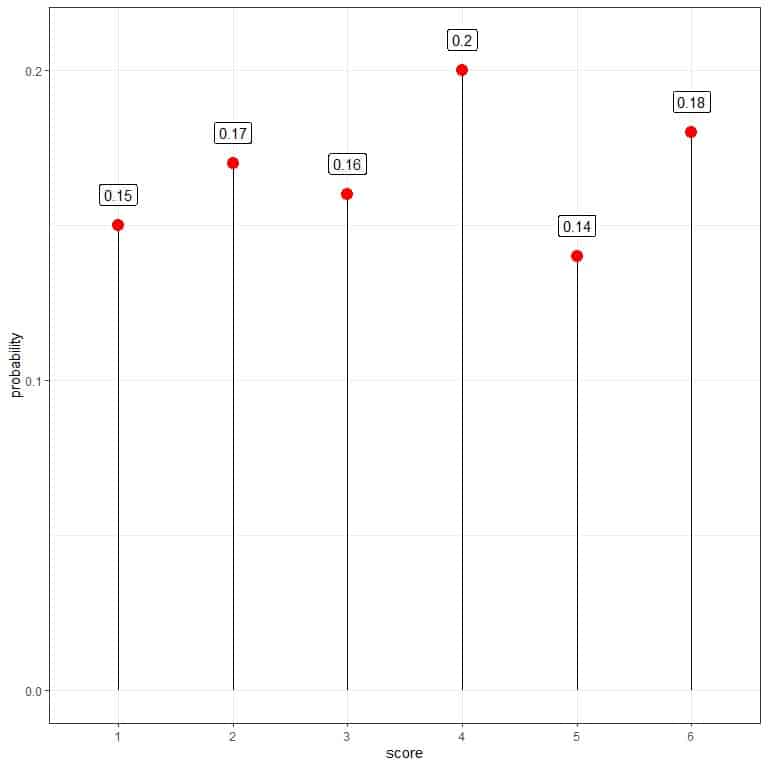
It is a likely fair die where the probability of every score is nearly identical.

– Example 3

You are checking the number of defective piston rings in a box of ten. As a quality check, you get 100 boxes, open them all, and count the number of defective units in each box.

The number of defective units is a random variable and can take values, 0,1,2,3,4,5,6,7,8,9, or 10. Zero means no defective units are found, and 10 means that all units in the box are defective.

You get the following results:

4 9 5 10 0 1 6 10 7 6 0 5 8 7 2 10 3 1 4 0 10 8 8 0 8 8 6 7 4 2 0 10 8 9 1 6 9 3 4 3 2 5 5 5 2 2 3 6 3 10 1 5 9 2 7 3 2 9 10 5 8 2 5 4 9 5 9 9 9 5 9 7 8 1 6 3 5 7 4 2 3 8 5 9 2 5 0 10 10 2 2 8 4 8 4 3 9 2 6 6.

In a table form:

From the table, we see that:

• The sum of the frequency column = 100, which is our sample size.
• The frequency of 0 is 6, meaning that 6 boxes have no defective units. On the other hand, the frequency of 10 is 9, meaning that there are 9 boxes where all their pistons were defective.

You can use that data to estimate the probability mass function for the number of defectives per box.

The probability for zero defectives = 6/100 = 0.06.

The probability for one defective = 5/100 = 0.05, and so on.

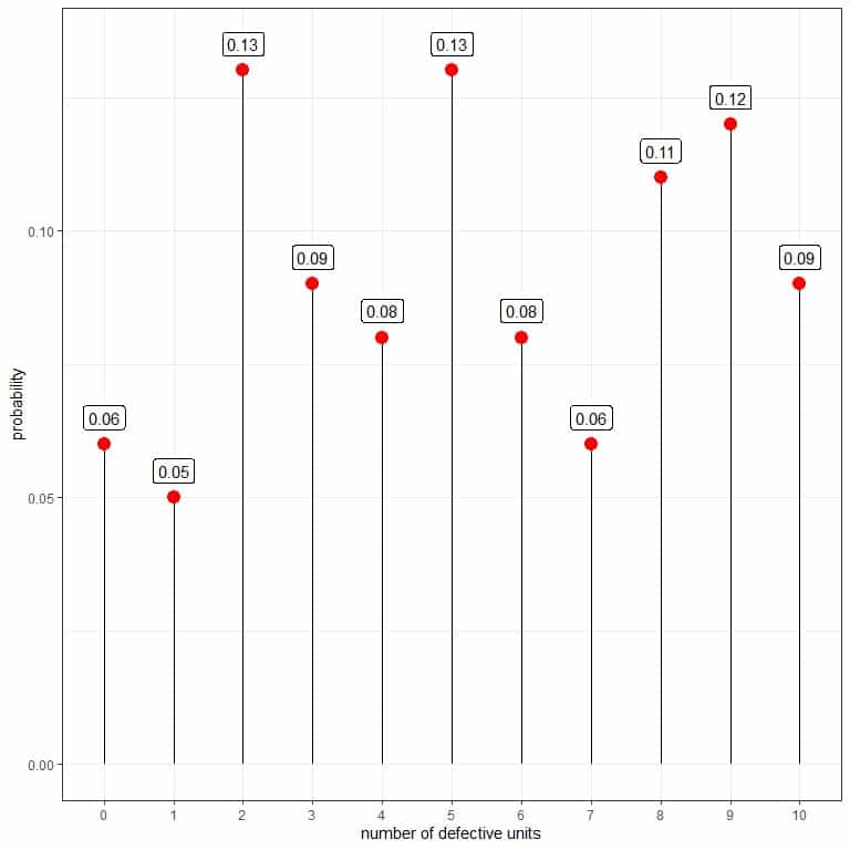
The probability that the number of defectives is equal to 0, 1, or 2 is the sum of the 3 probabilities for the 3 numbers = 0.06+0.05+0.13 = 0.24 or 24%.

The probability that the number of defectives is greater than 5 is the sum of the probabilities for numbers greater than 5 = 0.08+0.06+0.11+0.12+0.09 = 0.46 or 46%.

We see that this is a bad sample with many defectives so you requested a machine adjustment.

After this adjustment, you sampled another 100 boxes and get the following results for the number of defective:

1 5 2 6 7 0 3 7 3 2 8 2 4 3 0 7 1 0 1 8 6 4 4 9 4 4 3 3 1 0 8 7 4 5 0 2 5 1 1 1 0 2 2 2 0 0 1 2 1 6 0 2 5 0 3 1 0 5 7 2 4 0 2 1 5 2 5 5 5 2 5 4 4 0 2 1 2 3 2 0 1 4 2 5 0 2 9 7 6 0 0 4 1 4 1 1 5 0 2 3.

In a table form:

You can use that data to estimate the probability mass function for the number of defectives per box after machine adjustment.

The probability for zero defectives = 18/100 = 0.18.

The probability for one defective = 16/100 = 0.16, and so on.

Although 10 is a possible outcome, no box has all its units as defectives, so its probability is 0 and is not represented in the table.

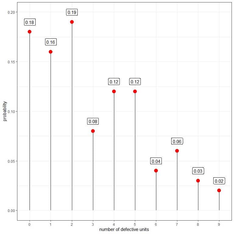
The probability that the number of defectives is greater than 5 is the sum of the probabilities for numbers greater than 5 = 0.04+0.06+0.03+0.02 = 0.15 or 15% compared to 46% before machine adjustment.

We conclude that there is a considerable improvement in our process.

Continuous random variable

Continuous random variables take an infinite number of possible values within a certain range and can take decimal values. Continuous random variables are usually measurements

Examples of continuous random variables: Height, weight, age, the time required to walk a mile, etc.

For example, a certain weight can be 70.5 kg. Still, with increasing balance accuracy, we can have a value of 70.5321458 kg. So the weight can take infinite values with infinite decimal places.

Since there is an infinite number of values in any interval, it is not meaningful to talk about the probability that the random variable will take on a specific value. Instead, the probability that a continuous random variable will lie within a given interval is considered.

Suppose the probability of a certain interval is high. In that case, this means that the continuous random variable can take the values within this interval with high probability and vice versa.

– Example 1

The following are the heights of 200 individuals from a certain survey.

160.0 163.0 170.0 147.0 158.0 164.0 154.5 160.0 160.0 163.0 160.0 167.0 150.0 156.0 157.0 180.0 163.0 155.0 156.0 162.0 155.5 155.0 158.5 172.0 174.0 161.0 153.0 169.0 167.0 170.0 159.0 164.5 169.0 160.0 158.0 162.0 158.0 174.0 149.0 148.0 156.0 178.0 156.0 167.0 165.0 151.0 155.0 160.0 151.5 165.0 155.0 158.0 167.0 173.0 177.0 165.0 155.0 152.0 155.0 161.3 174.0 172.0 145.0 167.5 159.0 153.4 147.5 151.5 180.0 182.0 149.0 148.0 151.0 153.0 152.0 171.0 158.0 143.0 172.0 158.0 171.0 169.0 166.0 155.0 171.0 150.5 162.0 162.0 167.0 157.0 145.0 163.0 165.0 175.0 158.9 181.0 158.0 177.0 169.0 165.0 148.0 150.0 161.0 152.0 164.5 182.0 174.5 157.0 171.0 140.0 167.2 161.0 182.0 160.5 143.0 168.0 166.0 167.0 180.0 158.5 155.0 171.0 157.0 157.0 161.0 162.0 168.5 146.0 147.0 162.0 158.0 162.0 178.0 170.0 164.0 152.0 167.0 158.0 151.0 155.0 165.0 180.0 162.5 176.0 173.0 159.0 159.5 175.0 170.0 183.0 171.0 161.0 158.0 164.0 171.2 161.0 178.5 157.0 163.0 150.0 165.5 156.0 160.4 168.0 164.0 160.2 167.0 144.0 156.0 155.0 143.0 175.0 156.0 162.0 164.0 164.0 151.0 162.0 162.0 166.0 184.0 169.0 166.0 153.5 144.0 153.0 164.0 160.0 171.0 170.0 159.0 175.0 172.0 169.0 178.0 157.0 152.3 162.0 156.5 151.0.

You can use that data to estimate the probability density function for the heights from the population from which this sample was taken.

1. Determine the number of bins you need.

The number of bins is log(observations)/log(2).

In this data, the number of bins = log(200)/log(2) = 7.6 will be rounded up to become 8.

2. Sort the data and subtract the minimum data value from the maximum data value to get the data range.

The sorted data will be:

140.0 143.0 143.0 143.0 144.0 144.0 145.0 145.0 146.0 147.0 147.0 147.5 148.0 148.0 148.0 149.0 149.0 150.0 150.0 150.0 150.5 151.0 151.0 151.0 151.0 151.0 151.5 151.5 152.0 152.0 152.0 152.0 152.3 153.0 153.0 153.0 153.4 153.5 154.5 155.0 155.0 155.0 155.0 155.0 155.0 155.0 155.0 155.0 155.0 155.5 156.0 156.0 156.0 156.0 156.0 156.0 156.0 156.5 157.0 157.0 157.0 157.0 157.0 157.0 157.0 158.0 158.0 158.0 158.0 158.0 158.0 158.0 158.0 158.0 158.0 158.5 158.5 158.9 159.0 159.0 159.0 159.0 159.5 160.0 160.0 160.0 160.0 160.0 160.0 160.0 160.2 160.4 160.5 161.0 161.0 161.0 161.0 161.0 161.0 161.3 162.0 162.0 162.0 162.0 162.0 162.0 162.0 162.0 162.0 162.0 162.0 162.5 163.0 163.0 163.0 163.0 163.0 164.0 164.0 164.0 164.0 164.0 164.0 164.0 164.5 164.5 165.0 165.0 165.0 165.0 165.0 165.0 165.5 166.0 166.0 166.0 166.0 167.0 167.0 167.0 167.0 167.0 167.0 167.0 167.0 167.2 167.5 168.0 168.0 168.5 169.0 169.0 169.0 169.0 169.0 169.0 170.0 170.0 170.0 170.0 170.0 171.0 171.0 171.0 171.0 171.0 171.0 171.0 171.2 172.0 172.0 172.0 172.0 173.0 173.0 174.0 174.0 174.0 174.5 175.0 175.0 175.0 175.0 176.0 177.0 177.0 178.0 178.0 178.0 178.5 180.0 180.0 180.0 180.0 181.0 182.0 182.0 182.0 183.0 184.0.

In our data, the minimum value is 140, and the maximum value is 184, so:

The range = 184 – 140 = 44.

3. Divide the data range in Step 2 by the number of classes you get in Step 1. Round the number, you get up to a whole number to get the class width.

Class width = 44 / 8 = 5.5. Rounded up to 6.

4. Add the class width, 6, sequentially (8 times because 8 is the number of bins) to the minimum value to create the different 8 bins.

140 + 6 = 146 so the first bin is 140-146.

146 + 6 = 152 so the second bin is 146-152.

152 + 6 = 158 so the third bin is 152-158.

158 + 6 = 164 so the fourth bin is 158-164.

164 + 6 = 170 so the fifth bin is 164-170.

170 + 6 = 176 so the sixth bin is 170-176.

176 + 6 = 182 so the seventh bin is 176-182.

182 + 6 = 188 so the eighth bin is 182-188.

5. We draw a table of 2 columns. The first column carries the different bins of our data that we created in step 4.

The second column will contain the frequency of heights in each bin.

• The bin “140-146” contains heights from 140 to 146.
• The next bin, “146-152,” contains heights larger than 146 to 152, and so on.

By looking at the sorted data in step 2, we see that:

• The first 9 numbers (140.0, 143.0, 143.0, 143.0, 144.0, 144.0, 145.0, 145.0, 146.0) are within the first bin “140-146” so the frequency of this bin is 9.
• The next 23 numbers (147.0, 147.0, 147.5, 148.0, 148.0, 148.0, 149.0, 149.0, 150.0, 150.0, 150.0, 150.5, 151.0, 151.0, 151.0, 151.0, 151.0, 151.5, 151.5, 152.0, 152.0, 152.0, 152.0) are within the second bin “146-152” so the frequency of this bin is 23.
• And so on till completing the frequency of all bins.
• If you sum these frequencies, you will get 200 which is the total number of data.

9+23+43+49+37+23+14+2 = 200.

6. Add a third column for the relative frequency or probability.

Relative frequency = frequency/total data number.

• All probabilities are >= 0 and sum to 1.
• The first bin, “140-146,” contains 9 data points or frequency, so the relative frequency of this bin = 9/200 = 0.04.
• The second bin, “146-152,” contains 23 data points or frequency, so the relative frequency of this bin = 23/200 = 0.12.

If you sum these relative frequencies, you will get nearly 1 (due to rounding):

0.04+0.12+0.22+0.24+0.18+0.12+0.07+0.01 = 1.

7. Use the table to plot a relative frequency histogram, where the data bins or ranges on the x-axis and the relative frequency (or proportions or probabilities) on the y-axis.

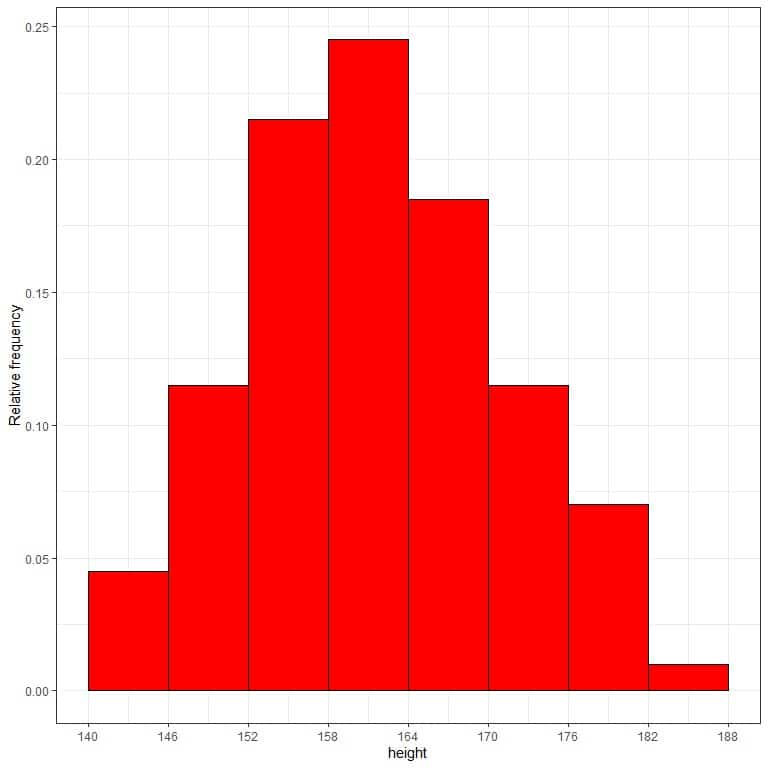
• In relative frequency histograms, we can interpret the heights or proportions as probabilities. We can use these probabilities to determine the likelihood of certain results occurring within a given interval.
• For example, the relative frequency of the “140-146” bin is 0.04, so the probability of heights falling in this range is 0.04 or 4%. On the other hand, the relative frequency of the “146-152” bin is 0.12. So the probability of heights to fall in this interval is 0.12 or 12%.
• It means that heights in the range “146-152” tend to occur more frequently than the heights in the range 140-146 from that population.

8. Add another column for the density.

Density = relative frequency/class width = relative frequency/6.

9. Suppose we decreased the intervals more and more. In that case, we could represent the probability distribution as a curve by connecting the “dots” at the tops of the tiny, tiny, tiny rectangles.

The area of this histogram or density plot is still 1.0.

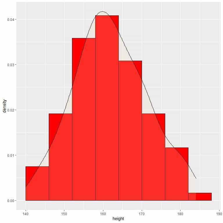
We see that most heights from this population are around 160 cm. As we go shorter or longer than 160 cm, the probability (or density) of heights decreases.

To convert density to probability, we integrate the density curve within a certain interval (or multiply the density by the interval width).

For example, the probability that heights are within 158-164 cm = density X6 = 0.04 X 6 = 0.24 or 24%.

Practice questions

1. You threw the die 100 times and get the following probability mass function:

What is the probability that the score will be 1?

What is the probability that the score will be 3?

Is that a fair die?

2. The following is the probability mass function for the hours per day watching TV for 150 persons (we consider hours as a discrete outcome, so no decimals are allowed):

What is the probability that persons are watching TV for larger than 10 hours/day?

What is the probability that persons are watching TV for 4 or fewer hours/day?

3. The following is the number of children per family, represented as a probability distribution for 500 families:

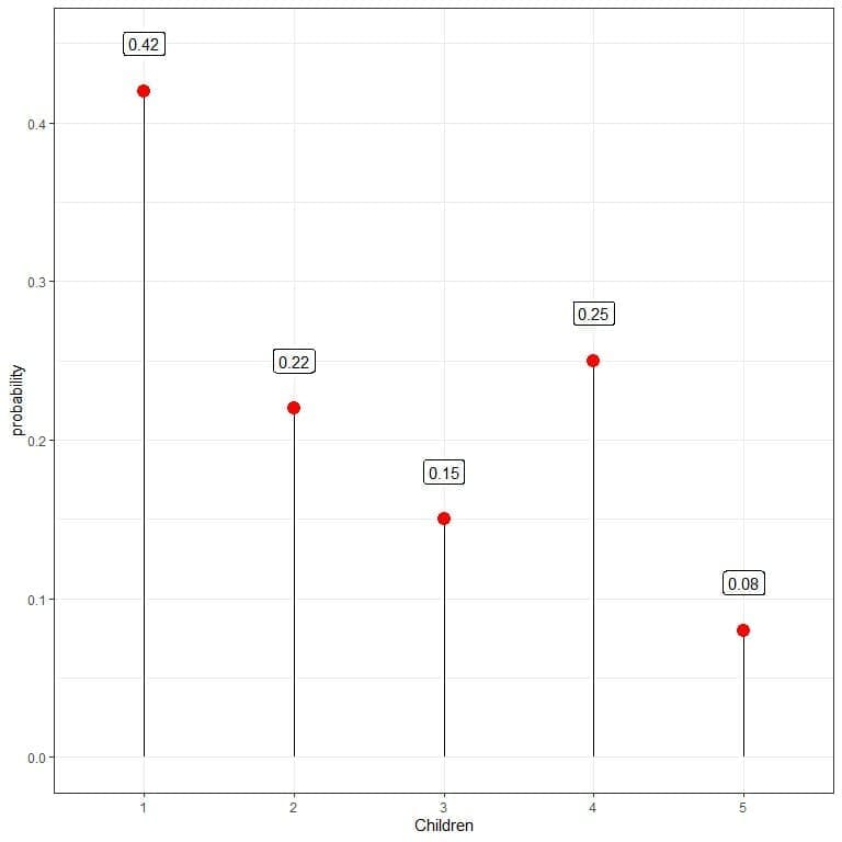What is the probability that families are having 4 children?

What is the probability that families are having 6 children?

What is wrong with this probability distribution?

4. The following is the density plots for the distribution of pressures for different storms:

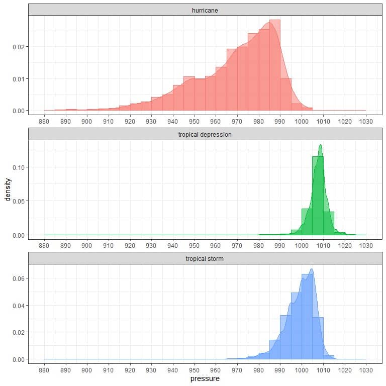
What is the most frequent interval for pressures from hurricanes, tropical depressions, and tropical storms?

5. The following are the density plots for the distribution of body mass index (BMI) for the two genders from a certain survey.

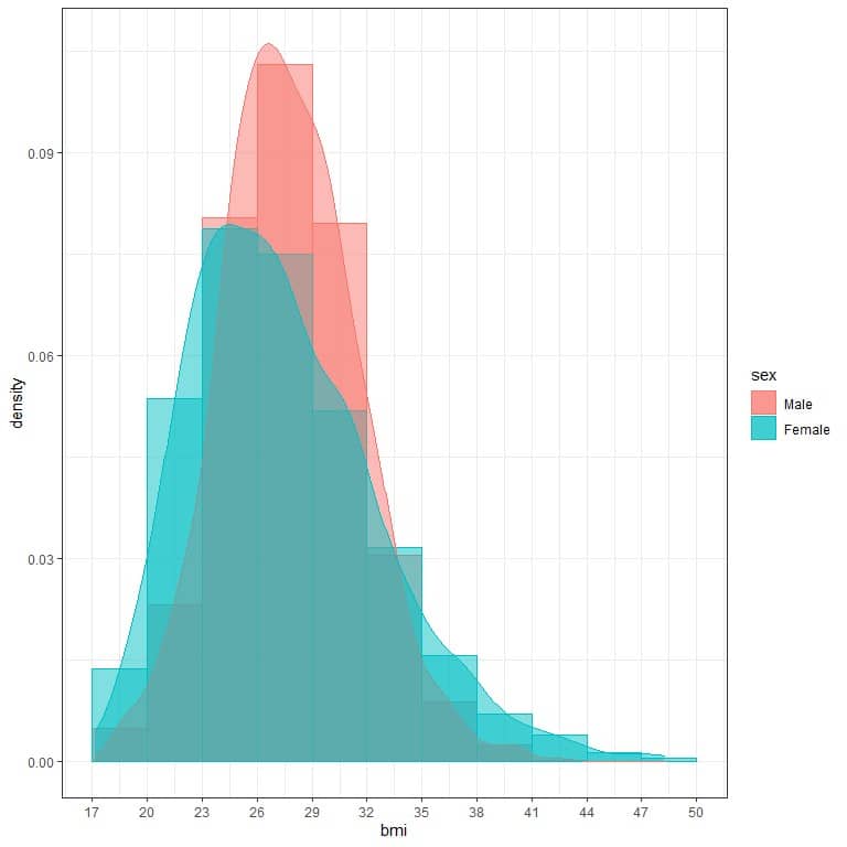
And the following table is the maximum BMI for each gender:

Although in the plot, the peak value for males is higher than the peak value for females, the maximum value for females is higher than that for males, why?

Answer key

1. The probability of 1 score = 0.04 or 4%.

The probability of 3 score = 0.46 or 46%.

It is not a fair die as scores 5 and 6 do not appear. Furthermore, there is a great variation in the probabilities of the 4 remaining scores.

2. The probability that persons are watching TV for larger than 10 hours/day = sum of probabilities for numbers greater than 10 = 0.027 or 2.7%.

The probability that persons are watching TV for 4 or less hours/day = sum of probabilities for numbers ≤ 4 = 0.087+0.127+0.160+0.133+0.04 = 0.547 or 54.7%.

3. From the plot, the probability that families are having 4 children = 0.25 or 25%.

The probability that families are having 6 children = zero since it is not represented in the plot.

The probability distribution is wrong because if we sum the probabilities, we get a number larger than 1 = 0.42+0.22+0.15+0.25+0.08 = 1.12.

4. We look at the peak of every plot or the highest rectangle of each histogram:

For hurricanes, values between 985-990.

For tropical depression, values between 1005-1010.

For tropical storms, values between 1000-1005.

5. The peak value of the density plot represents the most frequent BMI in males or females.

A higher peak for males means that the 26-29 value for BMI is more frequent in males than in females.

The tail of every density plot represents the maximum.

The blue curve for females is more tailed to the right than the red curve for males, so females’ maximum BMI is higher than that for males.

Previous Lesson | Main Page | Next Lesson