JUMP TO TOPIC
Tangent Plane – Definition, Equation, and Examples
The tangent plane allows us to predict the behaviors of surfaces at certain points of the function. Through this article, we’ll see how partial derivatives come in handy when studying functions in space and approximating linear functions to model the behavior of curves at certain points. In the 2D coordinate system, we studied tangent lines, so in space, we’ll have to master the concept of tangent planes.
The tangent plane is an extension of the tangent line in three-dimensional coordinate systems. To find the equation of the tangent plane, we’ll need to approximate a linear equation using the partial derivatives of the function.
Our discussion will cover the fundamental concepts behind tangent planes. We’ll also show you how the formula was established. Of course, we’ll make sure that by the end of the article, you’ll feel confident in finding the tangent planes of different curves!
What Is a Tangent Plane?
The tangent plane represents the surface that contains all tangent lines of the curve at a point, $P$, that lies on the surface and passes through the point. In our earlier discussions of derivatives and tangent lines, we’ve learned that we can approximate the behavior of a graph using tangent lines. Now that we’re working with multivariable functions and three-dimensional coordinate systems, we can use tangent planes for a similar purpose.
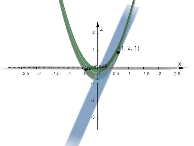
Here’s an example of the curve of $z = 3x^2 – xy$ graphed in green with its tangent plane, $z = 4x – y – 1$. As you can see from the graph, the tangent plane covers the point, $(1, 2,1)$. From this, we can see that the curve and its tangent plane behave similarly at the point, $(1, 2,1)$. This means that through tangent planes, we can now observe the behavior of the function’s curve at a given point.
As with tangent lines in a 2D coordinate system, we have a process to establish so that we can find the tangent plane’s equation smoothly.
Understanding the Tangent Plane Formula
Suppose that $f(x)$ is a continuous partial derivatives, we can think of the tangent plane to the surface, $z = f(x, y)$, and passes through the point, $P(x_o, y_o, z_o)$ as the surface that contains all the tangent lines passing through $P$. We’ve learned in the past that we can write the equation as
\begin{aligned}A(x – x_o) + B(y – y_o) + C(z – z_o) = 0\end{aligned}
Keep in mind that $\textbf{n} = \left<A, B, C \right>$ is a vector that is normal to the tangent plane. Now, let’s divide both sides of the plane’s equation by $C$ then isolate $z – z_o$ on the left-hand side of the equation shown below.
\begin{aligned}\dfrac{A}{C}(x – x_o) + \dfrac{B}{C}(y – y_o) + \dfrac{C}{C}(z – z_o) &= 0\\\dfrac{A}{C}(x – x_o) + \dfrac{B}{C}(y – y_o) + (z – z_o) &= 0\\\\z -z_o = -\dfrac{A}{C}(x – x_o) – \dfrac{B}{C}(y – y_o)\end{aligned}
If we let $a = – \dfrac{A}{C}$ and $b = – \dfrac{B}{C}$, we have the simplified equation:
\begin{aligned} z – z_o &= a(x – x_o) + b(y – y_o)\end{aligned}
If we’re working with the two tangent lines, $T_1$ and $T_2$, where they intersect the curve at $y = y_o$ and $x = x_o$, respectively. Hence, we have the following equations for the tangent lines, $T_1$ and $T_2$:
\begin{aligned}\boldsymbol{T_1}\end{aligned} | \begin{aligned}\boldsymbol{T_2}\end{aligned} |
\begin{aligned}z – z_o &= a(x – x_o)\end{aligned} | \begin{aligned}z – z_o &= b(y – y_o)\end{aligned} |
Both equations are in their point-slope forms where $a$ and $b$ represent the slope of the tangents. But since these represent the tangent lines, we know that $a = f_x(x_o, y_o)$ and $b = f_y(x_o, y_o)$. This establishes the general form of the tangent plane:
EQUATION OF THE TANGENT PLANE When $f$ has continuous partial derivatives, there exists an equation of the tangent plane to the surface, $z = f(x, y)$, that passes through the point, $P(x_o, y_o, z_o)$. We can write the tangent plane’s equation as shown below: \begin{aligned}z – z_o &= f_x(x_o, y_o)(x – x_o) + f_y(x_o, y_o)(y – y_o) \end{aligned} |
Keep in mind that $f_x(x, y)$ and $f_y(x, y)$ represent the partial derivatives of $f(x,y )$ with respect to $x$ and $y$, respectively. This means that the slopes, $f_x(x_o, y_o)$ and $f_y(x_o, y_o)$, are simply the partial derivatives of $f(x,y)$ evaluated at $(x_o, y_o)$.
Now that we’ve established the general form of the equation of the tangent plane, let’s go ahead and see how we can use this equation to find different equations of tangent planes to our given curves.
How To Find a Tangent Plane?
Use the general form of the equation of the tangent plane to guide you in establishing the equation of the plane tangent to the curve. Here are some pointers to remember when doing so:
- Take the partial derivatives of the function.
- Evaluate each partial derivative, $f_x(x,y )$ and $f_y(x, y)$, at $(x_o, y_o)$.
- Use $P(x_o, y_o, z_o)$ and the partial derivatives evaluated at $(x_o, y_o)$ to write the equation of the tangent plane.
\begin{aligned}z – z_o &= f_x(x_o, y_o)(x – x_o) + f_y(x_o, y_o)(y – y_o) \end{aligned}
Let us show you how to apply these steps by finding the tangent plane to the hyperbolic paraboloid, $z = x^2 –y^2$, at the point $(-2, 1, 2)$. First, let’s evaluate the partial derivatives of the surface as shown below.
\begin{aligned}\boldsymbol{f_x(x,y) = \dfrac{\partial f}{\partial x}}\end{aligned} | \begin{aligned}\dfrac{\partial f}{\partial {\color{Teal}x}} ({\color{Teal} x^2} – y^2) &= ({\color{Teal}2x}) – 0\\&= 2x\end{aligned} |
\begin{aligned}\boldsymbol{f_y(x,y) = \dfrac{\partial f}{\partial y}}\end{aligned} | \begin{aligned}\dfrac{\partial f}{\partial {\color{DarkOrange}y}} (x^2 – {\color{DarkOrange} y^2}) &= 0 – ({\color{DarkOrange}2y})\\&= -2y\end{aligned} |
Now, evaluate each of these partial derivatives at $x_o = -2$ and $y_o = 1$.
\begin{aligned}f_x(-2, 1)\end{aligned} | \begin{aligned}f_y(-2, 1)\end{aligned} |
\begin{aligned}f_x(-2, 1) &= 2(-2)\\&= -4\end{aligned} | \begin{aligned}f_y(-2, 1) &= -2(1)\\&= -2\end{aligned} |
Use $P(x_o, y_o, z_o) = (-2, 1, 2)$, $f_x(-2, 1) = -4$, and $f_y(-2, 1) = -2$ into the general form of the tangent plane’s equation as shown below.
\begin{aligned}z – z_o &= f_x(x_o, y_o)(x – x_o) + f_y(x_o, y_o)(y – y_o)\\ z – 2&= (-4)(x – – 2) + (-2)(y – 1)\\z – 2 &= -4(x + 2) – 2(y – 1) \end{aligned}
We can rearrange the equation by isolating $z$ on the left-hand side of the equation.
\begin{aligned}z – 2 &= -4x – 8 – 2y +2 \\z &= -4x – 8 – 2y +2 + 2\\z&= -4x – 2y -4\end{aligned}
This means that the equation of the tangent plane is $ z – 2 = -4(x + 2) – 2(y – 1)$ or $ z = -4x – 2y -4$.
Linear Approximation: Application of Tangent Planes
Through tangent planes, we can now approximate the linearization of functions. Notice how the resulting tangent plane returns a linear equation? We can use the resulting equation to approximate the linearization of the function at $(x_o, y_o)$.
This means that for $z = x^2 –y^2$, we can use the linear function, $ z = -4x – 2y -4$ to approximate the linearization of the hyperbolic paraboloid, $z = x^2 –y^2$.
\begin{aligned}f(x, y) \approx -4x – 2y -4\end{aligned}
The equation above is called the linear approximation of $f(x, y)$ at the point, $(-2, 1)$. This means that for points close to the value of $(-2, 1)$, the linear approximation can be used to approximate the value of the function.
We’ve covered all the important concepts that we need to be able to work on different problems involving tangent planes. Feel free to review the article once more and when you’re ready, head over to the problems we’ve prepared in the section below!
Example 1
Determine the equation of the tangent plane to the surface, $z = 12x^3y^2 – 4y$, at the point, $(-2, 2, -392)$.
Solution
To find the tangent plane at the point, $P(x_o, y_o, z_o) = (-2, 1, 4)$, we’ll need to evaluate the partial derivatives of the functions at $(x_o, y_o)$.
- Evaluate the partial derivative with respect to $x$ by treating the variable, $y$, as a constant.
- Apply a similar process to evaluate the partial derivative of the surface with respect to $y$ by treating $x$ as a constant.
We’ve summarized the calculations for you in the table below. The highlighted variable shows the variable we’re working on and leaving the remaining variable as a constant.
\begin{aligned}\boldsymbol{f_x(x,y) = \dfrac{\partial f}{\partial x}}\end{aligned} | \begin{aligned}\dfrac{\partial f}{\partial {\color{Teal}x}} (12{\color{Teal} x^3}y^2 – 4y)] &= 12({\color{Teal}3x^{3 – 1}})y^2 – 0\\&=12(3x^2y^2)\\&= 36x^2y^2\end{aligned} |
\begin{aligned}\boldsymbol{f_y(x,y) = \dfrac{\partial f}{\partial y}}\end{aligned} | \begin{aligned}\dfrac{\partial f}{\partial {\color{DarkOrange}y}} (12x^3{\color{DarkOrange} y^2} – {\color{DarkOrange}4y})] &= 12x^3({\color{DarkOrange}2y^{2 – 1}}) – {\color{DarkOrange}4(1)}\\&=12x^3(2y) – 4\\&= 24x^3y -4\end{aligned} |
Now that we have the expressions for $f_x(x, y)$ and $f_y(x,y)$, evaluate each expression at $x_o = -2$ and $y_o = 1$.
\begin{aligned}f_x(-2, 2)\end{aligned} | \begin{aligned}f_y(-2, 2)\end{aligned} |
\begin{aligned}f_x(-2, 2) &= 36(-2)^2(2)^2\\&= 36(4)(4)\\&= 576\end{aligned} | \begin{aligned}f_y(-2, 2) &= 24(-2)^3(2) -4\\&= 24(16) – 4\\&= 380\end{aligned} |
Use $P(x_o, y_o, z_o) = (-2, 2, 6)$, $f_x(-2, 2) = 576$, and $f_y(-2, 2) = 380$ into the general form of the tangent plane’s equation.
\begin{aligned}z – z_o &= f_x(x_o, y_o)(x – x_o) + f_y(x_o, y_o)(y – y_o)\\ z – 6 &= (576)(x – – 2) + (380)(y – 2)\\z – 6 &= 576(x + 2) – 380(y – 2) \end{aligned}
Arrange the equation to isolate $z$ on the left-hand side of the equation as shown below.
\begin{aligned}z + 392 &= 576x + 1144 – 380y + 760\\z&= 576x – 380 y – 392\end{aligned}
This means that the tangent plane of the surface at the point, $(-2, 2, 6)$, has the equation: $ z + 392 = 576(x + 2) – 380(y – 2)$ or $ z = 576x – 380 y + 1512$.
Example 2
Determine the equation of the tangent plane to the surface, $z = \ln(3x – 4y)$, at the point, $(7, 5)$.
Solution
As with our previous examples, we begin by taking the partial derivatives of the function 1) with respect to $x$ and 2) with respect to $y$. Use the derivative rule, $\dfrac{d}{dx} \ln x = \dfrac{1}{x}$, to evaluate the function’s partial derivatives.
\begin{aligned}\boldsymbol{f_x(x,y) = \dfrac{\partial f}{\partial x}}\end{aligned} | \begin{aligned}\dfrac{\partial f}{\partial {\color{Teal}x}} \ln(3{\color{Teal}x} – 4y) &={\color{Teal}\dfrac{1}{3x – 4y}} \cdot\dfrac{\partial f}{\partial {\color{Teal}x}} (3{\color{Teal}x} – 4y)\\&=\dfrac{1}{3x – 4y} \cdot [3({\color{Teal}1}) – 0]\\&= \dfrac{3}{3x – 4y}\end{aligned} |
\begin{aligned}\boldsymbol{f_y(x,y) = \dfrac{\partial f}{\partial y}}\end{aligned} | \begin{aligned}\dfrac{\partial f}{\partial {\color{DarkOrange}y}} \ln(3x – 4{\color{DarkOrange}y}) &={\color{DarkOrange}\dfrac{1}{3x – 4y}} \cdot\dfrac{\partial f}{\partial {\color{DarkOrange}y}} (3x – 4{\color{DarkOrange}y})\\&=\dfrac{1}{3x – 4y} \cdot [0 – 4({\color{DarkOrange}1})]\\&= -\dfrac{4}{3x – 4y}\end{aligned} |
Since the tangent plane passes through the point, $(5, 4)$, evaluate $f_x(x_o, y_o)$ and $f_y(x_o, y_o)$ at $x_o = 5$ and $y_o = 4$.
\begin{aligned}f_x(7, 5)\end{aligned} | \begin{aligned}f_y(7, 5)\end{aligned} |
\begin{aligned}f_x(7, 5) &= \dfrac{3}{3(7) – 4(5)}\\&= \dfrac{3}{21 – 20}\\&= 3\end{aligned} | \begin{aligned}f_y(7, 5) &= -\dfrac{4}{3(7) – 4(5)}\\&= -\dfrac{4}{21 – 20}\\&= -4\end{aligned} |
Now, before we plug in these values into the general form of the tangent plane’s equation, let’s first find the value of $z_o$ by evaluating $z = \ln(3x – 4y)$ at $x_o = 7$ and $y_o =5$.
\begin{aligned}z_o &= \ln( 3 \cdot 7 – 4 \cdot 5) \\&= \ln 1\\&= 0\end{aligned}
We now have all the values that we need, so let’s now write the tangent plane’s equation when it passes through the point, $(7, 5, 0)$.
\begin{aligned}z – z_o &= f_x(x_o, y_o)(x – x_o) + f_y(x_o, y_o)(y – y_o)\\ z – 0 &= (3)(x – 7) + (5)(y – 5)\\z &= 3(x – 7) + 5(y – 5) \end{aligned}
You can continue simplifying the right-hand side of the equation as shown below.
\begin{aligned}z &= 3x – 21 + 5y – 25\\z&= 3x + 5y – 46 \end{aligned}
Hence, the tangent plane of the surface at the point, $(7, 5, 0)$, has the equation: $z = 3(x – 7) + 5(y – 5) $ or $ z = 3x + 5y – 46 $.
Example 3
Determine the linear approximation to the curve, $z = 4 + \dfrac{x^2}{8} + \dfrac{y^2}{5}$ at $(-2, 4)$. Use the linear approximation to calculate $(-1.99, 4.01)$.
Solution
As we have learned in our discussion, we can use the tangent plane to form the linear approximate of the curve. This means that we’ll first find the equation representing the tangent plane, so let’s go ahead and evaluate the partial derivatives of the function.
\begin{aligned}\boldsymbol{f_x(x,y) = \dfrac{\partial f}{\partial x}}\end{aligned} | \begin{aligned}\dfrac{\partial f}{\partial {\color{Teal}x}} \left(4 + {\color{Teal}\dfrac{x^2}{8}} + \dfrac{y^2}{5} \right )&= 0 + {\color{Teal}2 \cdot \dfrac{1}{8}x^{2 -1 }} + 0\\&= \dfrac{x}{4}\end{aligned} |
\begin{aligned}\boldsymbol{f_y(x,y) = \dfrac{\partial f}{\partial y}}\end{aligned} | \begin{aligned}\dfrac{\partial f}{\partial {\color{DarkOrange}y}} \left(4 + \dfrac{x^2}{8} + {\color{DarkOrange}\dfrac{y^2}{5}} \right )&= 0 + 0 + {\color{DarkOrange}2 \cdot \dfrac{1}{5}y^{2 -1 }} \\&= \dfrac{2y}{5}\end{aligned} |
Let’s now find the values of $f_x(-2, 4)$ and $f_y(-2, 4)$.
\begin{aligned}f_x(-2, 4)\end{aligned} | \begin{aligned}f_y(-2, 4)\end{aligned} |
\begin{aligned}f_x(-2, 4) &= \dfrac{-2}{4}\\&= -\dfrac{1}{2} \end{aligned} | \begin{aligned}f_y(-2, 4) &= \dfrac{2(4)}{5}\\&= \dfrac{8}{5} \end{aligned} |
We’ll need to evaluate $z$ as well before we can apply the formula for the tangent plane.
\begin{aligned}z&= 4 + \dfrac{x^2}{8} + \dfrac{y^2}{5}\\z_o &= 4 + \dfrac{(-2)^2}{8} + \dfrac{(4)^2}{5}\\&= 4 + \dfrac{1}{2} + \dfrac{16}{5}\\&= \dfrac{77}{10}\end{aligned}
Now, let’s write the tangent plane’s equation as shown below.
\begin{aligned}z – z_o &= f_x(x_o, y_o)(x – x_o) + f_y(x_o, y_o)(y – y_o)\\ z – \dfrac{77}{10} &= -\dfrac{1}{2}(x – -2) + \dfrac{8}{5}(y – 4)\\z – 7.7 &= -0.5(x + 2) + 1.6(y – 4) \end{aligned}
As we have mentioned, we can use the tangent plane to write a linear approximation for the surface. Hence, we have the following linear approximation:
\begin{aligned}z &= -0.5x – 1 + 1.6y – 6.4 + 7.7\\z&= -0.5x + 1.6y + 0.3\\\\L(x,y) &\approx -0.5x + 1.6y + 0.3\end{aligned}
Hence, the linear approximation of the curve is $L(x, y) = -0.5x + 1.6y + 0.3$.
To approximate the value of the function at $(-1.99, 4.01)$, evaluate the linear approximation at $x = -1.99$ and $y = 4.01$.
\begin{aligned} L(-1.99, 4.01) &\approx -0.5(-1.99) + 1.6(4.01) + 0.3\\&\approx 7.711\end{aligned}
This shows that we can estimate values of the function at complex values using the linear approximation. Hence, we have $L(-1.99, 4.01) \approx 7.711$.
Practice Questions
1. Determine the equation of the tangent plane to the surface, $z = 2x^2y + 4xy$, at the point, $(1, 1,6)$.
2. Determine the equation of the tangent plane to the surface, $z = \ln(5x + 3y)$, at the point, $(2, -3)$.
3. Determine the linear approximation to the curve, $z = 4 + \dfrac{x^2}{6} + \dfrac{y^2}{9}$ at $(-4, 3)$. Use the linear approximation to calculate $(-4.01, 2.99)$.
Answer Key
1. $z – 6 = 8(x – 1) + 6(y – 1)$ or $z = 8x + 6y – 8$
2. $z = 5(x – 2) + 3(y + 3)$ or $z = 5x + 3y -1$
3. $L(x, y) \approx 5 – \dfrac{1}{2}(x + 4) + \dfrac{2}{3}(y – 3)$; $L(-4.01, 2.99) \approx 4.998$
3D images/mathematical drawings are created with GeoGebra.