Vector Function – Definition, Properties, and Explanation
The
vector functions allow us to visualize functions in two or three-dimensional coordinate systems and account for another element: the direction of the curve. Similar to parametric functions, vector functions depend on parameters to visualize their graphs. These functions are most helpful when we’re observing different types of curvatures.
What makes a vector function or vector-valued function special is that its input values are real numbers, yet its output is a set of vectors. Vector functions are extremely helpful when we want to visualize curves in space while accounting for the curves’ directions. In this article, we’ll cover the fundamental definition of a vector function. We’ll also show you how to evaluate and graph different types of vector functions. Refresh your knowledge on
parametric curves and the
three-dimensional coordinate system.Are you ready? Let’s dive right into understanding what makes vector functions unique!
What Is a Vector Function?
Vector functions or vector-value functions are functions that have
real set of numbers as their domain while the
range returns a set of vectors. Vector functions can have multiple dimensions, but we will limit our discussion on vectors with two or three dimensions:
| Vector Functions in Two Dimensions | \begin{aligned}\textbf{r}(t) &= x(t) \textbf{i} + y(t) \textbf{j}\end{aligned} |
| Vector Functions in Three Dimensions | \begin{aligned}\textbf{r}(t) &= x(t) \textbf{i} + y(t) \textbf{j} + z(t) \textbf{k}\end{aligned} |
As with other parametric functions, we normally use $t$ to represent the parameter since one of the most common parameters used is time. Here are some other ways we can write vector-valued functions:
| Vector Functions in Two Dimensions | \begin{aligned}\textbf{r}(t) &= <x(t), y(t)>\end{aligned} |
| Vector Functions in Three Dimensions | \begin{aligned}\textbf{r}(t) &= <x(t) ,y(t), z(t)> \end{aligned} |
We call $x(t)$, $y(t)$, and $z(t)$ as the components of the vector function, $\textbf{r}(t)$. In our discussion, we’ll focus on vector functions that contain three -dimensional vectors. One example of a vector function is $\textbf{r} = 3\cos t \textbf{i} + 3\sin t \textbf{i} + t \textbf{k}$ with its graph shown below.
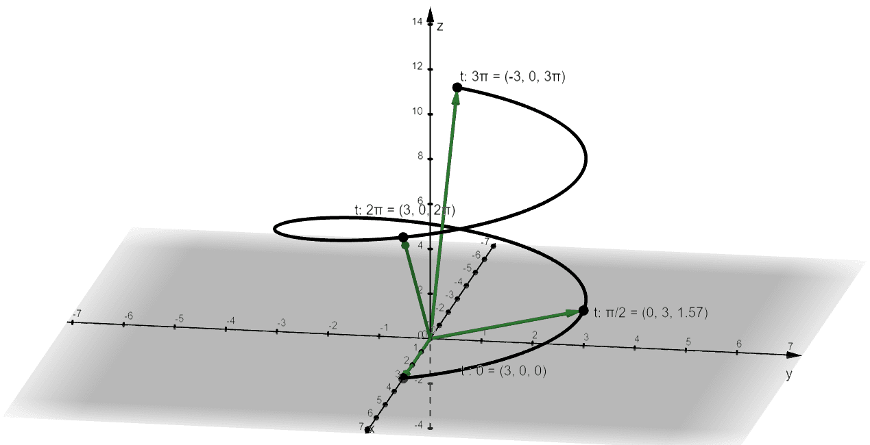
The graph shows that the resulting values are vectors such as the vector,$\textbf{r}(0) = <3, 0, 0>$ or $3 \textbf{i}$. These vectors will highlight the behavior of the curve in space at different values of $t$.
- When $t = \dfrac{\pi}{2}$, we have the vector, $\left<0, 3, \dfrac{\pi}{2}\right> = 3\textbf{j} + \dfrac{\pi}{2} \textbf{k}$.
- When $t = 2\pi$, we have the vector, $\left<3, 0, 2\pi\right> = 3\textbf{i} + 2\pi \textbf{k}$.
- When $t = 3\pi$, we have the vector, $\left<-3, 0,32\pi\right> = -3\textbf{i} + 3\pi \textbf{k}$.
We can define the domain of $\textbf{r}(t)$ by finding the intersection of the individual components of the vector function. This means that when we have $\textbf{r} = <\sqrt{1- t}, t^2, e^t>$, we can find the vector function’s domain using the domain of each of the component. Find the intersection of these three domains to determine the domain of $\textbf{r}(t)$.
| Component | Domain |
| \begin{aligned}x(t) = \sqrt{1 – t}\end{aligned} | \begin{aligned} t \geq 1\end{aligned} |
| \begin{aligned}y(t) = t^2\end{aligned} | \begin{aligned} -\infty < t < \infty \end{aligned} |
| \begin{aligned}z(t) = e^t\end{aligned} | \begin{aligned} -\infty < t < \infty \end{aligned} |
| Domain of Vector Function: $t \leq 1$ |

Here’s the graph of the vector function, $\textbf{r}(t) = <\sqrt{1- t}, t^2, e^t>$. This means that the function will be defined as long as $t \leq 1$. The range of the vector function reflects all the vectors formed from $\textbf{r}(t)$.
How To Solve a Vector Function?
When solving a problem involving vector functions, keep in mind that each component of the vector function represents a function in terms of a common parameter, $t$. Apply fundamental concepts learned in the past whenever needed.
Evaluating Vector FunctionsWhen evaluating the vector function at different values of $t$, we simply evaluate the functions, $x(t)$, $y(t)$, and $z(t)$. The value of the vector function will depend on the evaluated values of the components.For example, if we want to evaluate $\textbf{r} = <\sqrt{1- t}, t^2, e^t>$ at $t = -3$, we’ll need to evaluate each component at $t = -3$.
| \begin{aligned}x(t) &= \sqrt{1 – t}\end{aligned} | \begin{aligned}x(-3) &= \sqrt{1 – -3}\\&= 2\end{aligned} |
| \begin{aligned}y(t) &= t^2\end{aligned} | \begin{aligned}y(-3) &= (-3)^2\\&= 9\end{aligned} |
| \begin{aligned}z(t) &= e^t\end{aligned} | \begin{aligned}z(-3) &= e^{-3}\\&= \dfrac{1}{e^3}\end{aligned} |
Use the values of $x(-3)$, $y(-3)$, and $z(-3)$ to write the components of $\textbf{r}(-3)$. Hence, we have the following:\begin{aligned}\textbf{r}(-3) &= 2\textbf{i} + 3\textbf{j} + \dfrac{1}{e^3} \textbf{k}\\&= \left<2, 3, \dfrac{1}{e^3}\right>\end{aligned}Knowing how to evaluate vector functions correctly will make it easier for us when we need to graph the curve of the vector functions in two or three-dimensional coordinate system.
Evaluating Vector Functions’ LimitsWe can evaluate the limits of different vector functions, $\textbf{r}$, by evaluating the limits of each of the components.
| When $\textbf{r}(t) = <x(t), y(t), z(t)>$, we can express $\lim_{t \rightarrow a} \textbf{r} (t)$ as shown below:\begin{aligned}\lim_{t \rightarrow a} \textbf{r} (t) &= \left<\lim_{t \rightarrow a} x (t), \lim_{t \rightarrow a} y (t), \lim_{t \rightarrow a} z (t)\right>\end{aligned}This is true as long as the limits of each of the component functions exist. |
Evaluate the limits of $\textbf{r}(t)$’s component functions by applying the
limit laws we have applied in real-valued functions. Here are some of the most common limit properties you’ll be applying to find the vector functions’ limits:
| Properties of Limits |
| When $\textbf{r}_1(t) = \textbf{L}_1$ and $\textbf{r}_2(t) = \textbf{L}_2$, we can apply the following properties of limits:\begin{aligned}&(1)\phantom{x} \lim_{t \rightarrow a} k \cdot \textbf{r}_1(t) = k \cdot \textbf{L}_1, k\textbf{ is scalar}\\&(2)\phantom{x} \lim_{t \rightarrow a} [\textbf{r}_1(t) + \textbf{r}_2(t)] = \textbf{L}_1 + \textbf{L}_2 \\&(3)\phantom{x} \lim_{t \rightarrow a} [\textbf{r}_1(t) \cdot \textbf{r}_2(t)] = \textbf{L}_1 \cdot\textbf{L}_2\end{aligned} |
This means that when $\textbf{r}(t)$ is continuous at $a$, we have $\lim_{t \rightarrow a} \textbf{r}(t) = \textbf{r}(a)$.Let’s say we have $\textbf{r}(t) = \left<t^2, \dfrac{\sin(2t – 2)}{t – 2}, e^t\right>$, we can evaluate $\lim_{t \rightarrow 1} \textbf{r}(t)$ by taking the limit of $\textbf{r}(t)$’s components as $t \rightarrow 1$.
| \begin{aligned} \boldsymbol{\lim_{t \rightarrow 1} t^2} \end{aligned} | \begin{aligned} \lim_{t \rightarrow 1} t^2 &= (1)^2\\&= 1 \end{aligned} |
| \begin{aligned} \boldsymbol{\lim_{t \rightarrow 1} \dfrac{\sin(2t – 2)}{t – 2}} \end{aligned} | \begin{aligned} \lim_{t \rightarrow 1} \dfrac{\sin(2t – 2)}{t – 1} &= \dfrac{0}{0} \phantom{x}\Rightarrow\text{Use L’Hopital’s Rule}\\&= \lim_{r \rightarrow 1} \dfrac{2 \cos(2t – 2)}{1}\\&= 2\cos 0\\&= 2\end{aligned} |
| \begin{aligned} \boldsymbol{\lim_{t \rightarrow 1} e^t} \end{aligned} | \begin{aligned} \lim_{t \rightarrow 1} e^t &= (e)^1\\&= e \end{aligned} |
Using the limits of the components, we have $\lim_{t \rightarrow 1} \textbf{r}(t) = <1, 2, e>$.
Evaluating Vector Functions’ DerivativesFrom seeing how we evaluate the limits of vector functions, we can also conclude that we can evaluate the derivative of $\textbf{r}(t)$ by
differentiating each of the components.
| Suppose that $x(t)$, $y(t)$, and $z(t)$ are differentiable functions of $t$, we have the following:\begin{aligned}\textbf{r}(t) &= <x(t), y(t)> \\\textbf{r}\prime(t) &= <x\prime(t), y\prime(t)>\\\\\textbf{r}(t) &= <x(t), y(t), z(t)> \\ \textbf{r}\prime(t) &= <x\prime(t), y\prime(t), z\prime(t)>\end{aligned} |
Apply the
derivative rules we’ve learned in the past to simplify the derivative of each components. This means that when we have $\textbf{r}(t) = <5t, 2t^2, 4t>$, we can find the vector-valued function’s derivative by differentiating $5t$, $2t^2$, and $4t$ at with respect to $t$.\begin{aligned}\textbf{r}(t) &= <5t, 2t^2, 4t>\\\textbf{r}\prime(t) &= \left<\dfrac{d}{dt} \phantom{x}(5t), \dfrac{d}{dt} \phantom{x}(2t^2), \dfrac{d}{dt} \phantom{x}(4t)\right>\\&= <5(1), 2(2t^1), 4(1)>\\&= <5, 4t, 4>\end{aligned}Since derivatives of vectors and vector functions are one of the most applied concepts, we’ve created an article for that. Head over to this
link if you want to learn more about vector derivatives.Now that we’ve learned how to evaluate vector functions, it’s time that we learn how to graph different types of vector functions.
How To Graph a Vector Function?
We’ve learned in the past that vectors contain magnitude and direction. Recall that when a vector has an initial point at the origin, it is considered situated in its
standard position. This is why when graphing the vector-valued functions, it will be easy for us to graph the vectors in their standard positions.
- When $\textbf{r}(t) = x(t) \textbf{i} + y(t) \textbf{j}$, the graph of the vector function is a plane curve.
- When $\textbf{r}(t) = x(t) \textbf{i} + y(t) \textbf{j} + z(t) \textbf{k}$, the graph of the vector function is a space curve.
When we represent these curves using a vector-valued function, we can call the process the
vector parametrization. The parameter, $t$, will show us the orientation of the plane or space curve. We apply a similar process as we have graphed
parametric curves in the past. We’ll know the direction of the curve based on the vectors as $t$ increases.Here are some guidelines to help you when graphing vector functions:
- Set up a table of values for the vector-valued function.
- Evaluate the values of $\textbf{r}(t)$ at different values of $t$.
- Graph these vectors at either the 2D or 3D coordinate plane.
- Take note of the curve’s direction.
Since we’ve learned how to graph plane curves in the past, we’ll focus our examples on graphing vector functions as space curves. We’ll begin by graphing $\textbf{r}(t) = <2\cos t , 2 \sin t, t>$ when $0 \leq t 3\pi$:
- Assign some key values for $t$: $\left\{0, \pi, 2\pi, 3\pi, 4\pi\right\}$. We chose these values because it’s easy to evaluate $\cos t$ and $\sin t$ at different multiples of $\pi$.
- Use these values to evaluate $\textbf{r}(t)$.
- Construct the vectors formed by the origin and the different values of $\textbf{r}(t)$.
- Graph the space curve using the vectors and name the graph formed whenever possible.
| \begin{aligned}\boldsymbol{t}\end{aligned} | \begin{aligned}\boldsymbol{2\cos t}\end{aligned} | \begin{aligned}\boldsymbol{2 \sin t}\end{aligned} | \begin{aligned}\boldsymbol{t}\end{aligned} |
| \begin{aligned}0\end{aligned} | \begin{aligned}2 \end{aligned} | \begin{aligned}0\end{aligned} | \begin{aligned}0\end{aligned} |
| \begin{aligned} \dfrac{\pi}{2}\end{aligned} | \begin{aligned} 0 \end{aligned} | \begin{aligned}2\end{aligned} | \begin{aligned} \dfrac{\pi}{2}\end{aligned} |
| \begin{aligned} \pi \end{aligned} | \begin{aligned} -2 \end{aligned} | \begin{aligned}0\end{aligned} | \begin{aligned} \pi \end{aligned} |
| \begin{aligned} \dfrac{3\pi}{2}\end{aligned} | \begin{aligned} 0 \end{aligned} | \begin{aligned}-2\end{aligned} | \begin{aligned} \dfrac{3\pi}{2}\end{aligned} |
| \begin{aligned} 2\pi \end{aligned} | \begin{aligned} 2 \end{aligned} | \begin{aligned}0\end{aligned} | \begin{aligned} 2\pi \end{aligned} |
| \begin{aligned} \dfrac{5\pi}{2}\end{aligned} | \begin{aligned} 0 \end{aligned} | \begin{aligned} 2\end{aligned} | \begin{aligned} \dfrac{5\pi}{2}\end{aligned} |
| \begin{aligned} 2\pi \end{aligned} | \begin{aligned} 2 \end{aligned} | \begin{aligned}0\end{aligned} | \begin{aligned} 2\pi \end{aligned} |
Let’s graph six vectors in standard positions that pass through the six points from the table of values.

Construct the graph by creating curves that pass through each vector. We begin at $t = 0$ and continue sketching the curve as $t$ increases by $\dfrac{\pi}{2}$.

Hence, we have the graph as shown above. We call this curve space the
helix – from its name, we expect the graph to exhibit a shape that looks like a corkscrew or a spiral staircase. Is it possible for us to know if the vector function may return a helix? Let’s try to convert $\textbf{r}(t) = <2\cos t , 2 \sin t, t>$ as equation in terms of $x$, $y$, and $z$.\begin{aligned} x&= 2\cos t\\ y &= 2\sin t\\\\ x^2 + y^2 &= (2\cos t)^2 + (2\sin t)^2 \\ &= 4\cos^2 t + 4\sin^2 t\\&= 4(\cos^2 t + \sin^2 t)\\ &= 4(1)\\ &= 4\end{aligned}This means that when $t = 0$, we have a circle with an equation of $x^2 + y^2 = 4$ lying on the $xy$-plane. Since we have $z = t$, we expect that the circles move as $t$ increases. This exhibits a helical shape that has a circular base with a radius of $2$ units.
Examples of Complex Graphs From Vector Functions
There are space curves that are more complicated to graph by hand. Thanks to our current graphing utilities and programs, it is now much easier to represent these curve spaces. Here’s an example of a curve space we call the
toroidal spiral.

This toroidal spiral, for example, is represented by the vector function, $\textbf{r} = <(3 + 15\sin t)\cos t, (3 + 15\sin t)\sin t, \cos 15t>$. From the alone, we can see that the curve space is formed by spirals with a hole at the center, hence the name of the curve space.Another interesting curve space would be the
trefoil knot. Let us show you the graph of the vector function, $\textbf{r} = <(4 + \cos 2t)\cos t, (4 + \cos 2t)\sin t, \sin 2t>$.

Just by seeing the graph, this space curve will be challenging to graph by hand since it contains complex knots for its curve. Thanks to modern technology, we can easily visualize curves like these!The third space curve we’ll show you is called the
twisted cubic – and by seeing the graph below, you’ll see why.

This is the twisted cubic formed by graphing the vector function, $\textbf{r}(t) = <t, t^2, t^3>$. Does the shape look familiar? That’s because the graph looks like the cubic function’s curve in the 2D Cartesian plane.

The three graphs above show us how the twisted cubic may appear in different angles and perspectives. This shows that no matter how simple the twisted cubic may appear, it becomes tricky when we graph them by hand.These are just three of the many complex graphs graphing systems can produce for us. It is important, however, that we know what these graphs represent to better understand and predict the behavior of these curvatures.For now, let’s try out different problems to deepen our understanding of vector functions.
Example 1Determine whether the following statements are true or false. If the statement is false, change the underlined word or phrase to make the statement true.a. When the
input of a function is a vector, the function is a vector function.b. When sketching vector-valued functions, graph the
vectors to guide us.c. The domain of vector functions is a set of
vectors.
SolutionLet’s break down each of the statements and recall what we know about vector functions. We know that the input of vector functions will be real numbers, but their output will always be vectors.a. Hence, the statement is
false, and we can change the word
input to output instead.When we evaluate $\textbf{r}(t)$ at different values of $t$, the resulting values are vector at standard positions. We use these vectors to guide us in graphing the vector function as a plane or curve space.b. This means that the statement is
true.As we have mentioned, the input of vector functions is always a set of real numbers. This means that the domain will be a set of real numbers for any vector functions.c. The statement is
false. We can make the statement true by changing the
vectors to real numbers.
Example 2Find the domain of the following vector functions:a. $\textbf{r}_1(t) = \left<t^2, \dfrac{1}{t – 2} \right>$
b. $\textbf{r}_2(t) = \left<\sin t,\dfrac{1}{t^2 – 9}, \sqrt{t – 2}\right>$
c. $\textbf{r}_3(t) = \left<t^2 – 4, \ln(16 – t^2), \sqrt{t – 6}\right>$
SolutionTo find the domain of a vector function, we simply determine the domain of each of the components then account for all their domains for the vector function’s actual domain.For the first vector function, $\left<t^2, \dfrac{1}{t – 2} \right>$, let’s work on $t^2$ and $\dfrac{1}{t – 2}$’ domains to find the domain of our vector function.
- The domain of any quadratic function is the set of all real numbers, so the domain of $t^2$ is $(-\infty, \infty)$.
- The only restriction for $\dfrac{1}{t – 2}$ occurs when $t – 2 = 0$, so the domain of the second component is $(-\infty, 2) \cup (2, \infty)$.
| Component | Domain |
| \begin{aligned}x(t) = t^2\end{aligned} | \begin{aligned} (-\infty, \infty)\end{aligned} |
| \begin{aligned}y(t) = \dfrac{1}{t – 2}\end{aligned} | \begin{aligned} (-\infty, 2) \cup (2, \infty ) \end{aligned} |
| Domain of Vector Function: $(-\infty, 2) \cup (2, \infty ) $ |
This means that as long as $t \neq 2$, $\left<t^2, \dfrac{1}{t – 2} \right>$ will be valid, so the domain of $\textbf{r}_1(t)$ is equal to $(-\infty, 2) \cup (2, \infty )$.Let’s apply a similar process to find the domain of $\textbf{r}_2(t) = \left<\sin t,\dfrac{1}{t^2 – 9}, \sqrt{t – 2}\right>$.
- The sine function has not restrictions for its input values, so the domain of $t$ is $(-\infty, \infty)$.
- The only restrictions for $\dfrac{1}{t^2 – 9}$ will occur when the denominator is zero, hence the domain of the second component is $(-\infty, -3) \cup (-3, 3) \cup (3, \infty)$.
- For $\sqrt{t – 2}$ to be valid, $t -2$ must be greater than or equal to zero, so the domain of the third component is $[2, \infty)$.
| Component | Domain |
| \begin{aligned}x(t) = \sin t\end{aligned} | \begin{aligned} (-\infty, \infty)\end{aligned} |
| \begin{aligned}y(t) = \dfrac{1}{t^2 – 9}\end{aligned} | \begin{aligned} (-\infty, -3) \cup (-3, 3) \cup (3, \infty)\end{aligned} |
| \begin{aligned}z(t) = \sqrt{t – 2}\end{aligned} | \begin{aligned} \left[2, \infty\right) \end{aligned} |
| Domain of Vector Function: $[2, 3) \cup (3, \infty ) $ |
After accounting for the domains of all three components, the domain of $\textbf{r}_2(t)$ is equal to $(2, 3) \cup (3, \infty ) $.Lastly, let’s work on the components of $\textbf{r}_3(t) = \left<t^2 – 4, \ln(t^2 – 16), \sqrt{t – 6}\right>$.
- Since $t^2 -4$ is a quadratic expression, its domain is all real numbers: $(-\infty, \infty)$.
- For $\ln(t^2 – 16)$, we need to make sure that $t^2 – 16$ is greater than zero, so its domain is $(-\infty, -4) \cup (4, \infty)$.
- The expression inside the square root must be greater than or equal to zero, so the domain of $\sqrt{t – 6}$ is $[6, \infty)$.
| Component | Domain |
| \begin{aligned}x(t) = t^2 -4 \end{aligned} | \begin{aligned} (-\infty, \infty)\end{aligned} |
| \begin{aligned}y(t) = \ln(t^2 – 16)\end{aligned} | \begin{aligned} (-\infty, -4) \cup (4, \infty) \end{aligned} |
| \begin{aligned}z(t) = \sqrt{t – 6}\end{aligned} | \begin{aligned} \left[6, \infty\right) \end{aligned} |
| Domain of Vector Function: $[6, \infty)$ |
Hence, we’ve shown that the domain of $\textbf{r}_3(t)$ is equal to $[6, \infty)$.
Example 3 For each of the following vector functions, find the values of $\textbf{r}( -4)$, $\textbf{r}(0)$, and $\textbf{r}(4)$.a. $\textbf{r}(t) = \left<t^2 – 1, \sqrt{t + 5} \right>$
b. $\textbf{r}(t) = \left<4t+ 1,\dfrac{1}{t^2 – 1}, \sqrt{6 – t}\right>$
c. $\textbf{r}(t) = \dfrac{1}{t – 1}\textbf{i} + \sin \pi t \textbf{j} + \ln(e^t)\textbf{k}$
SolutionFor each vector function, we can evaluate its values at $t = -4$, $t = 0$, and $t = 4$ by evaluating each of the components at these values of $t$. We’ll summarize the calculation for each vector function in a table.
| \begin{aligned}\boldsymbol{t}\end{aligned} | \begin{aligned}\boldsymbol{x(t)}\end{aligned} | \begin{aligned}\boldsymbol{y(t)}\end{aligned} | \begin{aligned}\boldsymbol{\textbf{r}(t)}\end{aligned} |
| \begin{aligned} t = -4\end{aligned} | \begin{aligned} t^2 – 1 &= (-4)^2 – 1\\&=15\end{aligned} | \begin{aligned} \sqrt{t + 5} &= \sqrt{-4 + 5} \\&=1\end{aligned} | \begin{aligned} \textbf{r}(t) &= \left<x(t), y(t)\right> \\&=\left<15, 1\right>\end{aligned} |
| \begin{aligned} t = 0\end{aligned} | \begin{aligned} t^2 – 1 &= (0)^2 – 1\\&= -1\end{aligned} | \begin{aligned} \sqrt{t+ 5} &= \sqrt{0 + 5} \\&=\sqrt{5}\end{aligned} | \begin{aligned} \textbf{r}(t) &= \left<x(t), y(t)\right> \\&=\left<-1, \sqrt{5}\right>\end{aligned} |
| \begin{aligned} t = 4\end{aligned} | \begin{aligned} t^2 – 1 &= (4)^2 – 1\\&= 15\end{aligned} | \begin{aligned} \sqrt{t+ 5} &= \sqrt{4 + 5} \\&= 3 \end{aligned} | \begin{aligned} \textbf{r}(t) &= \left<x(t), y(t)\right> \\&=\left<15, 3\right>\end{aligned} |
Apply the same process to evaluate $\textbf{r}(t) = \left<4t+ 1,\dfrac{1}{t^2 – 1}, \sqrt{6 – t}\right>$. This time, we’re working with a vector function that has three components, so add one more column for $z(t)$.
| \begin{aligned}\boldsymbol{t}\end{aligned} | \begin{aligned}\boldsymbol{x(t)}\end{aligned} | \begin{aligned}\boldsymbol{y(t)}\end{aligned} | \begin{aligned}\boldsymbol{y(t)}\end{aligned} | \begin{aligned}\boldsymbol{\textbf{r}(t)}\end{aligned} |
| \begin{aligned} t = -4\end{aligned} | \begin{aligned} 4t +1&= 4(-4) +1 1\\&=-15\end{aligned} | \begin{aligned} \dfrac{1}{t^2 -1} &= \dfrac{1}{(-4)^2 – 1}\\&=\dfrac{1}{8}\end{aligned} | \begin{aligned} \sqrt{6 – t} &= \sqrt{6 – (-4)}\\&= \sqrt{10}\end{aligned} | \begin{aligned} \textbf{r}(t) &= \left<x(t), y(t), z(t)\right> \\&=\left<-15, \dfrac{1}{8}, \sqrt{10}\right>\end{aligned} |
| \begin{aligned} t = 0\end{aligned} | \begin{aligned} 4t +1&= 4(0) +1 1\\&=1\end{aligned} | \begin{aligned} \dfrac{1}{t^2 -1} &= \dfrac{1}{(0)^2 – 1}\\&= -1 \end{aligned} | \begin{aligned} \sqrt{6 – t} &= \sqrt{6 – (0)}\\&= \sqrt{6}\end{aligned} | \begin{aligned} \textbf{r}(t) &= \left<x(t), y(t), z(t)\right> \\&=\left<1, -1, \sqrt{6}\right>\end{aligned} |
| \begin{aligned} t = 4\end{aligned} | \begin{aligned} 4t +1&= 4(4) +1 1\\&=17\end{aligned} | \begin{aligned} \dfrac{1}{t^2 -1} &= \dfrac{1}{(4)^2 – 1}\\&= \dfrac{1}{8} \end{aligned} | \begin{aligned} \sqrt{6 – t} &= \sqrt{6 – (4)}\\&= \sqrt{2}\end{aligned} | \begin{aligned} \textbf{r}(t) &= \left<x(t), y(t), z(t)\right> \\&=\left<17, \dfrac{1}{8}, \sqrt{2}\right>\end{aligned} |
The third vector function is written in the form, $x(t) \textbf{i} + y(t) \textbf{j} + z(t) \textbf{k}$, but we’ll be applying the same process – evaluating each component at $t = -4$, $t = 0$, and $t = 4$.
| \begin{aligned}\boldsymbol{t}\end{aligned} | \begin{aligned}\boldsymbol{x(t)}\end{aligned} | \begin{aligned}\boldsymbol{y(t)}\end{aligned} | \begin{aligned}\boldsymbol{y(t)}\end{aligned} | \begin{aligned}\boldsymbol{\textbf{r}(t)}\end{aligned} |
| \begin{aligned} t = -4\end{aligned} | \begin{aligned} \dfrac{1}{t – 1} &= \dfrac{1}{-4 – 1}\\&= -\dfrac{1}{5}\end{aligned} | \begin{aligned} \sin \pi t &= \sin -4\pi\\&= 0\end{aligned} | \begin{aligned} \ln e^t &= \ln e^{-4}\\&= -4\end{aligned} | \begin{aligned} \textbf{r}(t) &= x(t) \textbf{i} + y(t) \textbf{j} + z(t) \textbf{k}\\&= -\dfrac{1}{5} \textbf{i} – 4\textbf{k} \end{aligned} |
| \begin{aligned} t = 0\end{aligned} | \begin{aligned} \dfrac{1}{t – 1} &= \dfrac{1}{0 – 1}\\&= -1\end{aligned} | \begin{aligned} \sin \pi t &= \sin 0 \cdot\pi\\&= 0\end{aligned} | \begin{aligned} \ln e^0 &= \ln e^0\\&= 1\end{aligned} | \begin{aligned} \textbf{r}(t) &= x(t) \textbf{i} + y(t) \textbf{j} + z(t) \textbf{k}\\&= -1 \textbf{i} + \textbf{k} \end{aligned} |
| \begin{aligned} t = 4\end{aligned} | \begin{aligned} \dfrac{1}{t – 1} &= \dfrac{1}{4 – 1}\\&= \dfrac{1}{3}\end{aligned} | \begin{aligned} \sin \pi t &= \sin 4 \cdot\pi\\&= 0\end{aligned} | \begin{aligned} \ln e^4 &= \ln e^4\\&= 4\end{aligned} | \begin{aligned} \textbf{r}(t) &= x(t) \textbf{i} + y(t) \textbf{j} + z(t) \textbf{k}\\&= \dfrac{1}{3} \textbf{i} + 4 \textbf{k} \end{aligned} |
These three examples show us how straightforward it is for us to evaluate vector functions at different values of $t$. Apply the same process when asked to evaluate the values of different vector functions in the future.
Example 4Evaluate the limits of the following vector functions:a. $\lim_{t \rightarrow 2} \left<e^{t – 1}, \dfrac{t – 2}{t^2 -4}\right>$
b. $\lim_{t \rightarrow \infty} \left< \dfrac{2}{t^2}, e^{-2t}, \dfrac{t^2}{t^2 + 4t – 4}\right>$
c. $\lim_{t \rightarrow -3} \left(\dfrac{t+ 3}{t^2 – 9}\textbf{i} + \ln (1-t) \textbf{j} + \dfrac{t^2 + 5t + 18}{t^2 + 4t + 3} \textbf{k}\right)$
SolutionRecall that when we need to evaluate the limits of vector functions, we simply evaluate the limits of each component. Let’s apply this concept to find the limits of the three items.Let’s begin by evaluating $\lim_{t \rightarrow 2} \left<e^{t – 1}, \dfrac{t – 2}{t^2 -4}\right>$. Apply the limit laws and techniques that we’ve learned in the past to simplify the expressions for each components.
| \begin{aligned} \boldsymbol{\lim_{t \rightarrow 2} e^{t – 1}} \end{aligned} | \begin{aligned} \lim_{t \rightarrow 2} e^{t – 1} &= e^{2 – 1}\\&= e \end{aligned} |
| \begin{aligned} \boldsymbol{\lim_{t \rightarrow 2} \dfrac{t – 2}{t^2 -4}}\end{aligned} | \begin{aligned} \lim_{t \rightarrow 2} \dfrac{t – 2}{t^2 -4} &= \lim_{t \rightarrow 2} \dfrac{t -2}{(t – 2)(t + 2)}\\&= \lim_{t \rightarrow 2} \dfrac{\cancel{t -2}}{\cancel{(t – 2)}(t + 2)}\\&= \lim_{t \rightarrow 2} \dfrac{1}{t + 2}\\&= \dfrac{1}{4}\end{aligned} |
a. This means that $\lim_{t \rightarrow 2} \left<e^{t – 1}, \dfrac{t – 2}{t^2 -4}\right>$ is equal to $\left<e, \dfrac{1}{4}\right>$.We’ll apply a similar process to evaluate $\lim_{t \rightarrow \infty} \left< \dfrac{2}{t^2}, e^{-2t}, \dfrac{t^2}{t^2 + 4t – 4}\right>$.
| \begin{aligned} \boldsymbol{\lim_{t \rightarrow \infty} \dfrac{2}{t^2}} \end{aligned} | \begin{aligned} \lim_{t \rightarrow \infty} \dfrac{2}{t^2} &= \dfrac{2}{\infty}\\&= 0 \end{aligned} |
| \begin{aligned} \boldsymbol{\lim_{t \rightarrow \infty} e^{-2t}}\end{aligned} | \begin{aligned} \lim_{t \rightarrow \infty} e^{-2t} &= \lim_{t \rightarrow \infty} \dfrac{1}{e^{2t}}\\ &= \dfrac{1}{\infty}\\&=0\end{aligned} |
| \begin{aligned} \boldsymbol{\lim_{t \rightarrow \infty} \dfrac{t^2}{t^2 + 4t – 4}}\end{aligned} | \begin{aligned} \lim_{t \rightarrow \infty} \dfrac{t^2}{t^2 + 4t – 4} &= \lim_{t \rightarrow \infty}\dfrac{\dfrac{t^2}{t^2}}{\dfrac{t^2}{t^2} + \dfrac{4t}{t^2} – \dfrac{4}{t^2}}\\&= \lim_{t \rightarrow \infty} \dfrac{1}{1 + \dfrac{4}{t} – \dfrac{4}{t^2}}\\&= \dfrac{1}{1 + 0 – 0}\\&= 1\end{aligned} |
b. Hence, $\lim_{t \rightarrow \infty} \left< \dfrac{2}{t^2}, e^{-2t}, \dfrac{t^2}{t^2 + 4t – 4}\right>$ is equal to $\left<0, 0, 1\right>$.Let’s now work on $\lim_{t \rightarrow -3} \left(\dfrac{t+ 3}{t^2 – 9}\textbf{i} + \ln (1-t) \textbf{j} + \dfrac{t^2 + 5t + 18}{t^2 + 4t + 3} \textbf{k}\right)$ by distributing the operating to each of the term.
| \begin{aligned} \boldsymbol{\lim_{t \rightarrow -3} \dfrac{t+ 3}{t^2 – 9}} \end{aligned} | \begin{aligned}\lim_{t \rightarrow -3} \dfrac{t+ 3}{t^2 – 9} &= \lim_{t \rightarrow -3} \dfrac{t+ 3}{( t- 3)( t + 3)}\\&=\lim_{t \rightarrow -3} \dfrac{\cancel{t+ 3}}{( t- 3)\cancel{( t + 3)}}\\&= \lim_{t \rightarrow -3} \dfrac{1}{t -3}\\&= \dfrac{1}{-3-3}\\&= -\dfrac{1}{6}\end{aligned} |
| \begin{aligned} \boldsymbol{\lim_{t \rightarrow -3} \ln (1-t) }\end{aligned} | \begin{aligned}\lim_{t \rightarrow -3} \ln (1-t) &= \lim_{t \rightarrow -3} \ln[1 – (-3)]\\&= \lim_{t \rightarrow -3} \ln 4\\&= \ln 4\end{aligned} |
| \begin{aligned} \boldsymbol{\lim_{t \rightarrow -3} \dfrac{t^2 + 5t + 18}{t^2 + 4t + 3}} \end{aligned} | \begin{aligned}\lim_{t \rightarrow -3} \dfrac{t^2 + 5t + 18}{t^2 + 4t + 3} &= \lim_{t \rightarrow -3}\dfrac{(t + 3)(t + 6)}{(t + 1)(t + 3)}\\&= \lim_{t \rightarrow -3}\dfrac{\cancel{(t + 3)}(t + 6)}{(t + 1)\cancel{(t + 3)}}\\&= \lim_{t \rightarrow -3} \dfrac{t + 6}{t + 1}\\&= \dfrac{-3 + 6}{-3 + 1}\\&= -\dfrac{3}{2}\end{aligned} |
c. This shows that $\lim_{t \rightarrow -3} \left(\dfrac{t+ 3}{t^2 – 9}\textbf{i} + \ln (1-t) \textbf{j} + \dfrac{t^2 + 5t + 18}{t^2 + 4t + 3} \textbf{k}\right)$ is simply equal to $-\dfrac{1}{6}\textbf{i} + \ln 4 \textbf{j} – \dfrac{3}{2} \textbf{k}$.
Example 5Calculate the derivative of the following vector functions:a. $\textbf{r}(t) = \left< \sin 2t, e^{-3t}, \ln(t^2 – 4)\right>$
b. $\textbf{r}(t) = \cos 3t\textbf{i} + \sqrt{4t + 1} \textbf{j} + te^{-t} \textbf{k}$
SolutionSimilar to limits, we can calculate the derivative of vector functions by differentiating their respective components. Let’s begin$\textbf{r}(t) = \left< \sin 2t, e^{-3t}, \ln(t^2 – 4)\right>$ by taking the derivative of $\sin 2t$, $e^{-3t}$, and $\ln(t^2 – 4)$ as shown below.\begin{aligned}\textbf{r}(t) &= \left< \sin 2t, e^{-3t}, \ln(t^2 – 4)\right>\\\textbf{r}^\prime(t) &= \left<\dfrac{d}{dt}\phantom{x} 2\sin 2t,\dfrac{d}{dt}\phantom{x} e^{-3t}, \dfrac{d}{dt}\phantom{x}\ln(t^2 – 4)\right>\\&= \left<2 \cos 2t \cdot \dfrac{d}{dt}(2t),e^{-3t}\cdot \dfrac{d}{dt}(-3t), \dfrac{1}{t^2 – 4}\cdot \dfrac{d}{dt}(t^2 -4) \right>\\&= \left<2 \cos 2t, -3e^{-3t}, \dfrac{2t}{t^2 – 4} \right>\end{aligned}a. This means that $\textbf{r}\prime(t) = \left<2 \cos 2t, -3e^{-3t}, \dfrac{2t}{t^2 – 4} \right>$.Apply the same process to find the derivative of $\textbf{r}(t) = \cos 3t\textbf{i} + \sqrt{4t + 1} \textbf{j} + te^{-t} \textbf{k}$. Brush up on the common derivative rules when needed, but don’t worry, we’ve broken down the steps for you!\begin{aligned}\textbf{r}(t) &= \cos 3t \phantom{x}\textbf{i} + \sqrt{4t + 1} \phantom{x}\textbf{j} + te^{-t} \phantom{x}\textbf{k}\\\textbf{r}^\prime(t) &= \dfrac{d}{dt}(\cos 3t )\phantom{x}\textbf{i} + \dfrac{d}{dt}(\sqrt{4t + 1})\phantom{x}\textbf{j} + \dfrac{d}{dt}(te^{-t})\phantom{x}\textbf{k}\\&= (-\sin 3t )\dfrac{d}{dt}(3t)\phantom{x}\textbf{i} + \dfrac{1}{2}(4t + 1)^{\frac{1}{2}-1}\dfrac{d}{dt}(4t + 1)\phantom{x}\textbf{j} + \left[\dfrac{d}{dt}\left(t\right)e^{-t}+\dfrac{d}{dt}\left(e^{-t}\right)t \right]\phantom{x}\textbf{k}\\&= – 3\sin 3t\phantom{x}\textbf{i} + \dfrac{2}{\sqrt{4t + 1}}\phantom{x}\textbf{j} + (e^{-t}-e^{-t}t)\phantom{x}\textbf{k}\end{aligned}b. Hence, we have $\textbf{r}\prime(t) = – 3\sin 3t\phantom{x}\textbf{i} + \dfrac{2}{\sqrt{4t + 1}}\phantom{x}\textbf{j} + (e^{-t}-e^{-t}t)\phantom{x}\textbf{k}$.
Practice Questions
1. Find the domain of the following vector functions:
a. $\left<t^2, \dfrac{1}{t – 4} \right>$
b. $\left<\cos t,\dfrac{1}{t^2 – 25}, \sqrt{t – 16}\right>$
c. $\left<t^2 – 81, \ln(9 – t^2), \sqrt{t + 5}\right>$2. For each of the following vector functions, find the values of $\textbf{r}(-\pi)$, $\textbf{r}(0)$, and $\textbf{r}(\pi)$.
a. $\textbf{r}(t) = \left<t^2 – 1, 2t + 4\right>$
b. $\textbf{r}(t) = \left<\sin t, \cos t, \tan t\right>$
c. $\textbf{r}(t) = \sin \dfrac{t}{2}\textbf{i} + \cos^2 t \textbf{j} + 2\sin \dfrac{t}{4}\textbf{k}$3. Evaluate the limits of the following vector functions:
a. $\lim_{t \rightarrow 4} \left<e^{t – 2}, \dfrac{t – 4}{t^2 – 16}\right>$
b. $\lim_{t \rightarrow \infty} \left< \dfrac{3}{t^2}, 2e^{-4t}, \dfrac{t^4}{2t^4 + 6t^2 – 6t}\right>$
c. $\lim_{t \rightarrow -2} \left(\dfrac{t+ 4}{t^2 – 16}\textbf{i} + \ln (t^2 – 3) \textbf{j} + \dfrac{ t^2 + 6t + 8}{ t^2 + 5t + 6} \textbf{k}\right)$4. Calculate the derivative of the following vector functions:
a. $\textbf{r}(t) = \left< \cos 6t, 2e^{-4t}, \ln(t^4 + 1)\right>$
b. $\textbf{r}(t) = \cos 3t\textbf{i} + \sqrt{t^2 + 4} \textbf{j} + 4te^{-t} \textbf{k}$5. Sketch the curve space of the following vector functions:
a. $\textbf{r}(t) = \left< 4\sin t, 4\cos t, t\right>$
b. $\textbf{r}(t) = t\textbf{i} + 2t^2 \textbf{j} + 5 \textbf{k}$
Answer Key
1.
a. $(-\infty, 4) \cup (4, \infty)$
b. $[16, \infty)$
c. $(-3, 3)$2.
| \begin{aligned}\textbf{r}(-\pi) \end{aligned} | \begin{aligned}\textbf{r}(0) \end{aligned} | \begin{aligned}\textbf{r}(\pi) \end{aligned} |
| a. | \begin{aligned}\left<\pi^2 – 1, 2\pi + 4\right>\end{aligned} | \begin{aligned}\left<– 1, 4\right>\end{aligned} | \begin{aligned}\left<\pi^2 – 1, -2\pi + 4\right>\end{aligned} |
| b. | \begin{aligned}\left<0,-1 ,0 \right>\end{aligned} | \begin{aligned}\left<0,1 ,0 \right>\end{aligned} | \begin{aligned}\left<0,-1 ,0 \right>\end{aligned} |
| c. | \begin{aligned}-1 \textbf{i} + 1 \textbf{j} -\sqrt{2} \textbf{k} \end{aligned} | \begin{aligned}1 \textbf{j} + 2 \textbf{k} \end{aligned} | \begin{aligned}1 \textbf{i} + 1 \textbf{j} + \sqrt{2} \textbf{k} \end{aligned} |
3.
a. $\left<e^{2}, \dfrac{1}{8}\right> $
b. $\left< 0, 0, \dfrac{1}{2}\right>$
c. $\dfrac{1}{6}\textbf{i} + 2 \textbf{k}$
4.
a. $\textbf{r}\prime(t) = \left< -6\sin 6t, -8e^{-4t}, \dfrac{4t^3}{t^4 + 1}\right>$
b. $\textbf{r}\prime(t) = – 3\sin 3t\phantom{x}\textbf{i} + \dfrac{t}{\sqrt{t^2+4}}\phantom{x}\textbf{j} + 4\left(e^{-t}-e^{-t}t\right) \phantom{x}\textbf{k}$
5.
a.

b.
 3D images/mathematical drawings are created with GeoGebra.
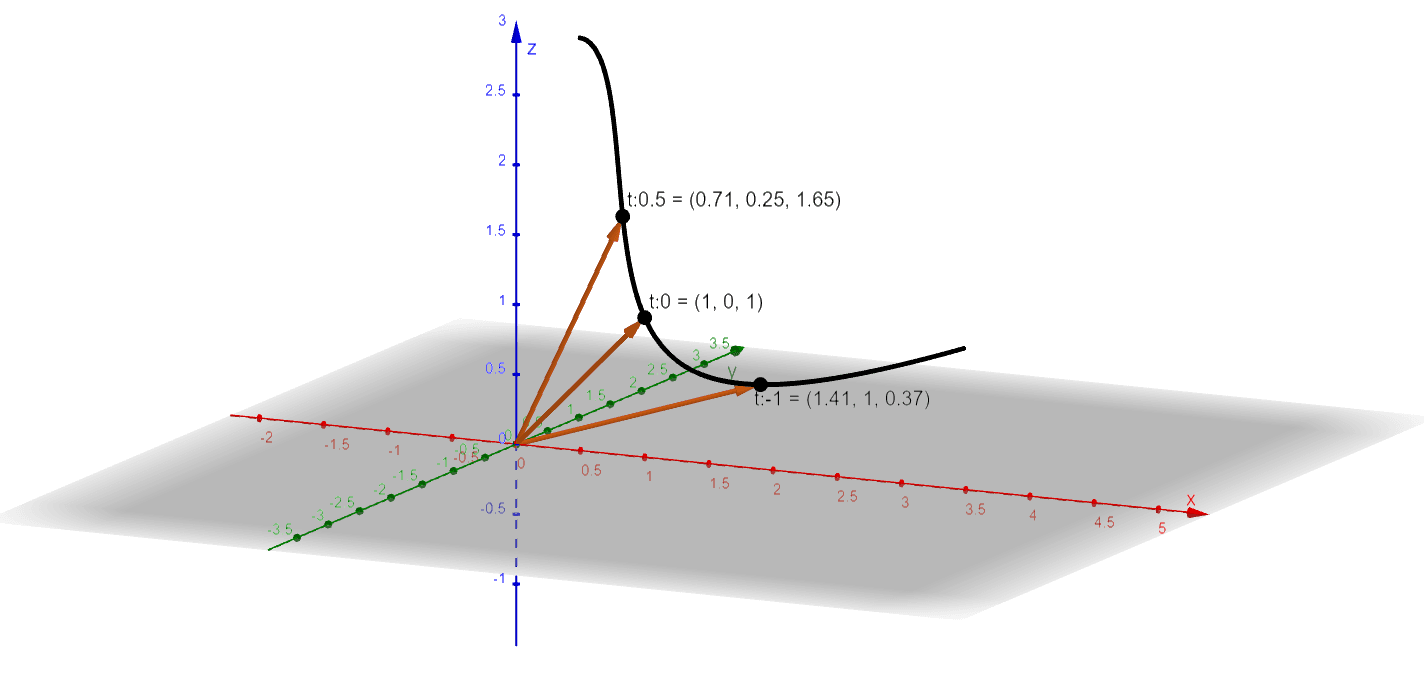 Here’s the graph of the vector function, $\textbf{r}(t) = <\sqrt{1- t}, t^2, e^t>$. This means that the function will be defined as long as $t \leq 1$. The range of the vector function reflects all the vectors formed from $\textbf{r}(t)$.
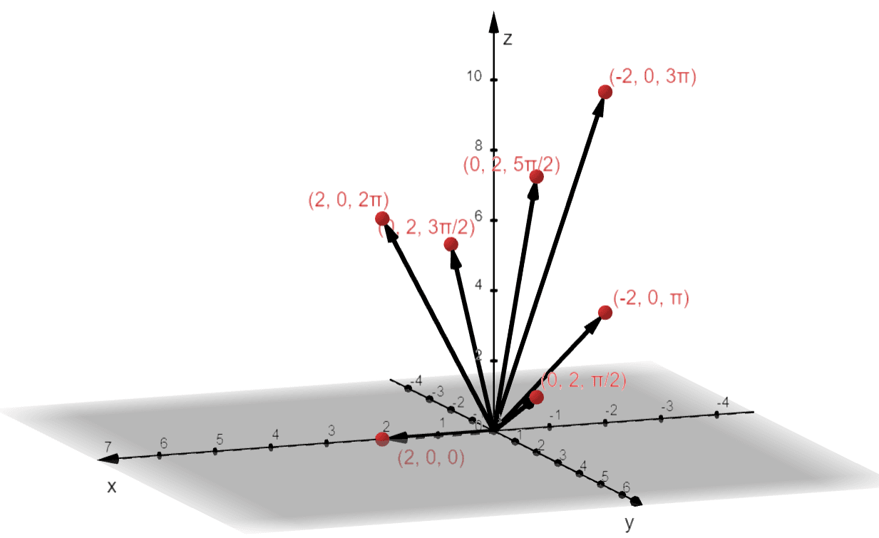 Construct the graph by creating curves that pass through each vector. We begin at $t = 0$ and continue sketching the curve as $t$ increases by $\dfrac{\pi}{2}$.
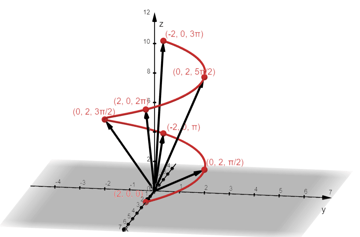 Hence, we have the graph as shown above. We call this curve space the helix – from its name, we expect the graph to exhibit a shape that looks like a corkscrew or a spiral staircase. Is it possible for us to know if the vector function may return a helix? Let’s try to convert $\textbf{r}(t) = <2\cos t , 2 \sin t, t>$ as equation in terms of $x$, $y$, and $z$.\begin{aligned} x&= 2\cos t\\ y &= 2\sin t\\\\ x^2 + y^2 &= (2\cos t)^2 + (2\sin t)^2 \\ &= 4\cos^2 t + 4\sin^2 t\\&= 4(\cos^2 t + \sin^2 t)\\ &= 4(1)\\ &= 4\end{aligned}This means that when $t = 0$, we have a circle with an equation of $x^2 + y^2 = 4$ lying on the $xy$-plane. Since we have $z = t$, we expect that the circles move as $t$ increases. This exhibits a helical shape that has a circular base with a radius of $2$ units.
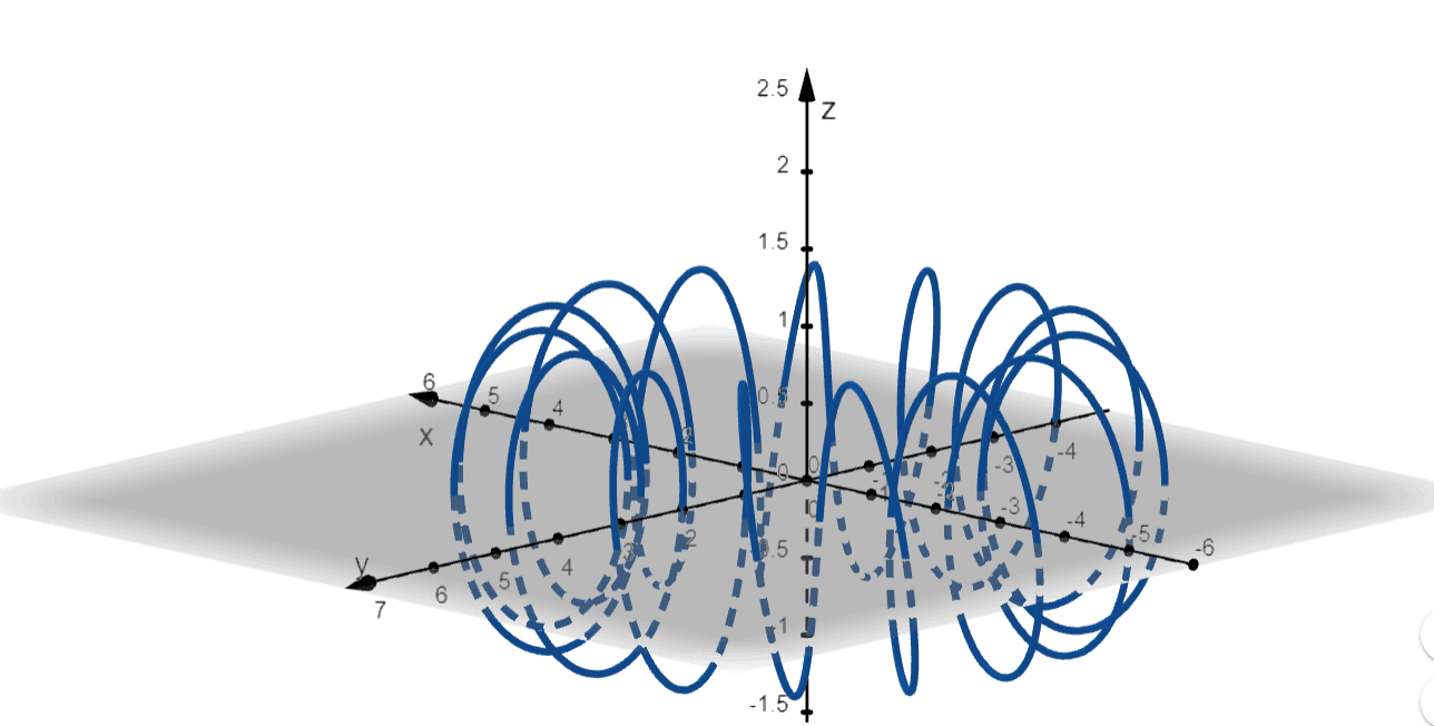 This toroidal spiral, for example, is represented by the vector function, $\textbf{r} = <(3 + 15\sin t)\cos t, (3 + 15\sin t)\sin t, \cos 15t>$. From the alone, we can see that the curve space is formed by spirals with a hole at the center, hence the name of the curve space.Another interesting curve space would be the trefoil knot. Let us show you the graph of the vector function, $\textbf{r} = <(4 + \cos 2t)\cos t, (4 + \cos 2t)\sin t, \sin 2t>$.
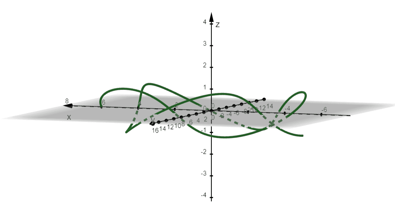 Just by seeing the graph, this space curve will be challenging to graph by hand since it contains complex knots for its curve. Thanks to modern technology, we can easily visualize curves like these!The third space curve we’ll show you is called the twisted cubic – and by seeing the graph below, you’ll see why.
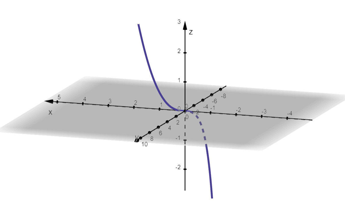 This is the twisted cubic formed by graphing the vector function, $\textbf{r}(t) = <t, t^2, t^3>$. Does the shape look familiar? That’s because the graph looks like the cubic function’s curve in the 2D Cartesian plane.
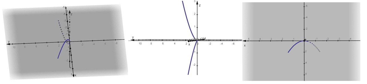 The three graphs above show us how the twisted cubic may appear in different angles and perspectives. This shows that no matter how simple the twisted cubic may appear, it becomes tricky when we graph them by hand.These are just three of the many complex graphs graphing systems can produce for us. It is important, however, that we know what these graphs represent to better understand and predict the behavior of these curvatures.For now, let’s try out different problems to deepen our understanding of vector functions.Example 1Determine whether the following statements are true or false. If the statement is false, change the underlined word or phrase to make the statement true.a. When the input of a function is a vector, the function is a vector function.b. When sketching vector-valued functions, graph the vectors to guide us.c. The domain of vector functions is a set of vectors.SolutionLet’s break down each of the statements and recall what we know about vector functions. We know that the input of vector functions will be real numbers, but their output will always be vectors.a. Hence, the statement is false, and we can change the word input to output instead.When we evaluate $\textbf{r}(t)$ at different values of $t$, the resulting values are vector at standard positions. We use these vectors to guide us in graphing the vector function as a plane or curve space.b. This means that the statement is true.As we have mentioned, the input of vector functions is always a set of real numbers. This means that the domain will be a set of real numbers for any vector functions.c. The statement is false. We can make the statement true by changing the vectors to real numbers.Example 2Find the domain of the following vector functions:a. $\textbf{r}_1(t) = \left<t^2, \dfrac{1}{t – 2} \right>$
b. $\textbf{r}_2(t) = \left<\sin t,\dfrac{1}{t^2 – 9}, \sqrt{t – 2}\right>$
c. $\textbf{r}_3(t) = \left<t^2 – 4, \ln(16 – t^2), \sqrt{t – 6}\right>$SolutionTo find the domain of a vector function, we simply determine the domain of each of the components then account for all their domains for the vector function’s actual domain.For the first vector function, $\left<t^2, \dfrac{1}{t – 2} \right>$, let’s work on $t^2$ and $\dfrac{1}{t – 2}$’ domains to find the domain of our vector function.
The three graphs above show us how the twisted cubic may appear in different angles and perspectives. This shows that no matter how simple the twisted cubic may appear, it becomes tricky when we graph them by hand.These are just three of the many complex graphs graphing systems can produce for us. It is important, however, that we know what these graphs represent to better understand and predict the behavior of these curvatures.For now, let’s try out different problems to deepen our understanding of vector functions.Example 1Determine whether the following statements are true or false. If the statement is false, change the underlined word or phrase to make the statement true.a. When the input of a function is a vector, the function is a vector function.b. When sketching vector-valued functions, graph the vectors to guide us.c. The domain of vector functions is a set of vectors.SolutionLet’s break down each of the statements and recall what we know about vector functions. We know that the input of vector functions will be real numbers, but their output will always be vectors.a. Hence, the statement is false, and we can change the word input to output instead.When we evaluate $\textbf{r}(t)$ at different values of $t$, the resulting values are vector at standard positions. We use these vectors to guide us in graphing the vector function as a plane or curve space.b. This means that the statement is true.As we have mentioned, the input of vector functions is always a set of real numbers. This means that the domain will be a set of real numbers for any vector functions.c. The statement is false. We can make the statement true by changing the vectors to real numbers.Example 2Find the domain of the following vector functions:a. $\textbf{r}_1(t) = \left<t^2, \dfrac{1}{t – 2} \right>$
b. $\textbf{r}_2(t) = \left<\sin t,\dfrac{1}{t^2 – 9}, \sqrt{t – 2}\right>$
c. $\textbf{r}_3(t) = \left<t^2 – 4, \ln(16 – t^2), \sqrt{t – 6}\right>$SolutionTo find the domain of a vector function, we simply determine the domain of each of the components then account for all their domains for the vector function’s actual domain.For the first vector function, $\left<t^2, \dfrac{1}{t – 2} \right>$, let’s work on $t^2$ and $\dfrac{1}{t – 2}$’ domains to find the domain of our vector function.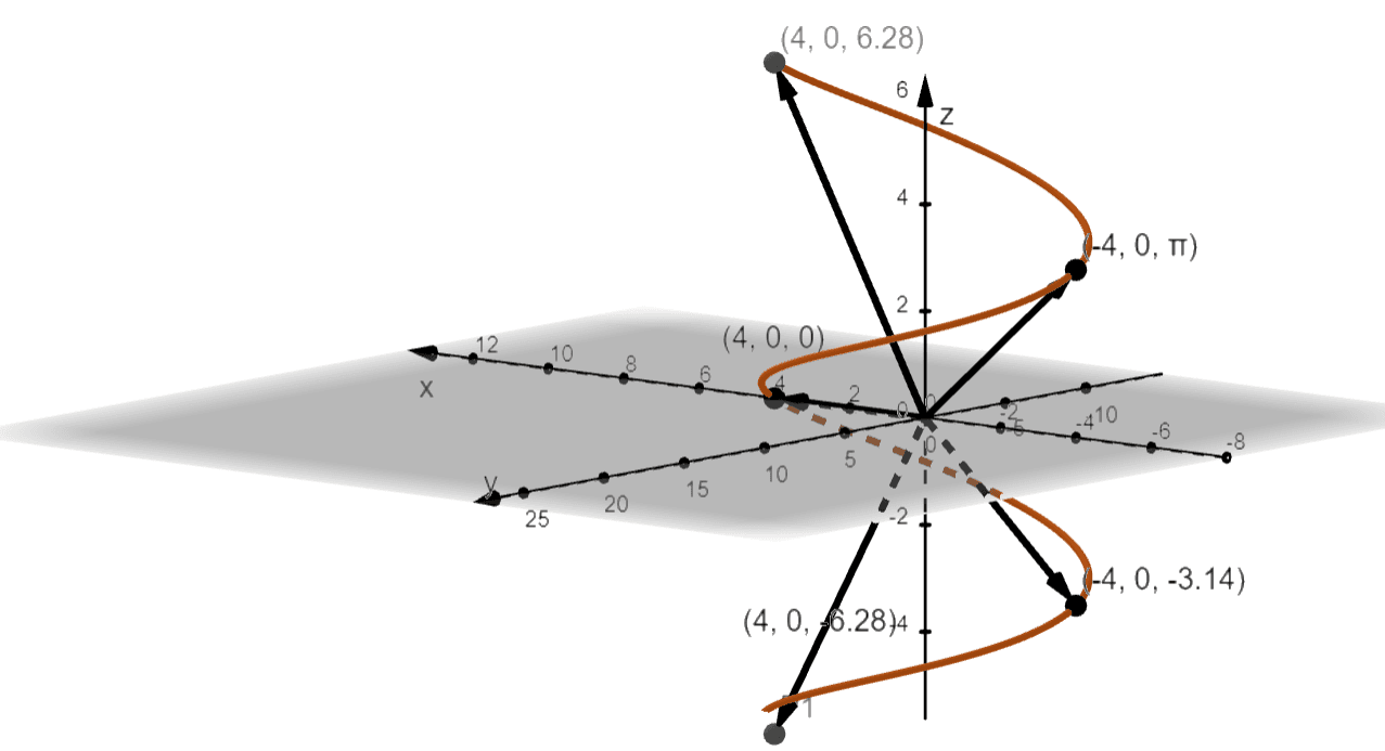 b.
b.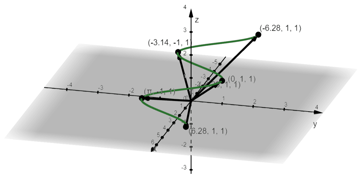 3D images/mathematical drawings are created with GeoGebra.