The Binomial Distribution – Explanation & Examples

The definition of the binomial distribution is:

“The binomial distribution is a discrete probability distribution that describes the probability of an experiment with only two outcomes.”

In this topic, we will discuss the binomial distribution from the following aspects:

• What is a binomial distribution?
• Binomial distribution formula.
• How to do the binomial distribution?
• Practice questions.
• Answer key.

What is a binomial distribution?

The binomial distribution is a discrete probability distribution that describes the probability from a random process when repeated multiple times.

For a random process to be described by the binomial distribution, the random process must be:

1. The random process is repeated a fixed number (n) of trials.
2. Each trial (or repetition of the random process) can result in only one of two possible outcomes. We call one of these outcomes a success and the other a failure.
3. The probability of success, denoted by p, is the same in every trial.
4. The trials are independent, meaning that one trial’s outcome does not affect the outcome in other trials.

Example 1

Suppose you are tossing a coin 10 times and count the number of heads from these 10 tosses. This is a binomial random process because:

1. You are tossing the coin only 10 times.
2. Each trial of tossing a coin can result in only two possible outcomes (head or tail). We call one of these outcomes (head, for example) a success and the other (tail) a failure.
3. The probability of success or head is the same in every trial, which is 0.5 for a fair coin.
4. The trials are independent, meaning that if the outcome in one trial is head, this does not allow you to know the outcome in subsequent trials.

In the above example, the number of heads can be:

• 0 meaning that you get 10 tails when tossing the coin 10 times,
• 1 meaning that you get 1 head and 9 tails when tossing the coin 10 times,
• 2 meaning that you get 2 heads and 8 tails,
• 3 meaning that you get 3 heads and 7 tails,
• 4 meaning that you get 4 heads and 6 tails,
• 5 meaning that you get 5 heads and 5 tails,
• 6 meaning that you get 6 heads and 4 tails,
• 7 meaning that you get 7 heads and 3 tails,
• 8 meaning that you get 8 heads and 2 tails,
• 9 meaning that you get 9 heads and 1 tail, or
• 10 meaning that you get 10 heads and no tails.

Using the binomial distribution can help us to calculate the probability of each number of successes. We get the following plot:

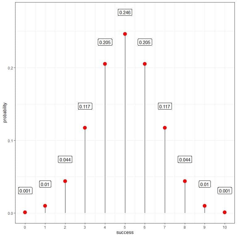As the probability of success is 0.5, so the expected number of successes in 10 trials = 10 trials X 0.5 = 5.

We see that 5 (meaning that we found 5 heads and 5 tails from these 10 trials) has the highest probability. As we move away from 5, the probability fades away.

We can connect the points to draw a curve:

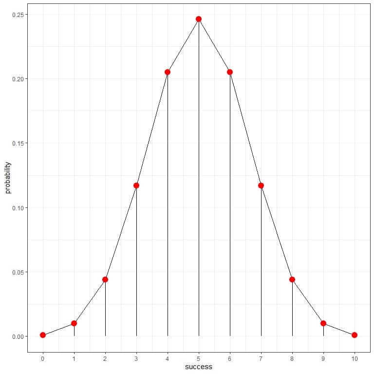This is an example of a probability mass function where we have the probability for each outcome. The outcome cannot take decimal places. For example, the outcome cannot be 3.5 heads.

Example 2

If you are tossing a coin 20 times and count the number of heads from these 20 tosses.

The number of heads can be 0,1,2,3,4,5,6,7,8,9,10,11,12,13,14,15,16,17,18,19, or 20.

Using the binomial distribution to calculate the probability of each number of successes, we get the following plot:

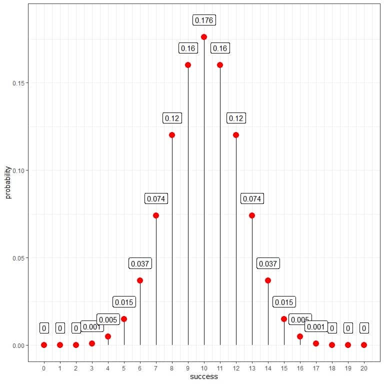As the probability of success is 0.5, so the expected successes = 20 trials X 0.5 = 10.

We see that 10 (meaning that we found 10 heads and 10 tails from these 20 trials) has the highest probability. As we move away from 10, the probability fades away.

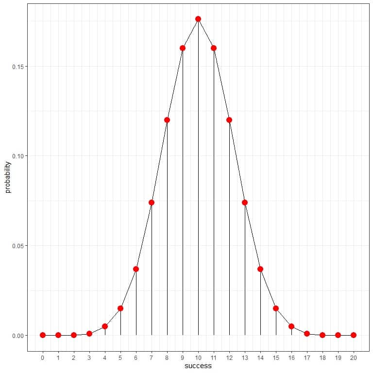
We can draw a curve connecting these probabilities:

The probability of 5 heads in 10 tosses is 0.246 or 24.6%, while the probability of 5 heads in 20 tosses is 0.015 or 1.5% only.

Example 3

If we have an unfair coin where the probability of a head is 0.7 (not 0.5 as the fair coin), you are tossing this coin 20 times and counting the number of heads from these 20 tosses.

The number of heads can be 0,1,2,3,4,5,6,7,8,9,10,11,12,13,14,15,16,17,18,19, or 20.

Using the binomial distribution to calculate the probability of each number of successes, we get the following plot:

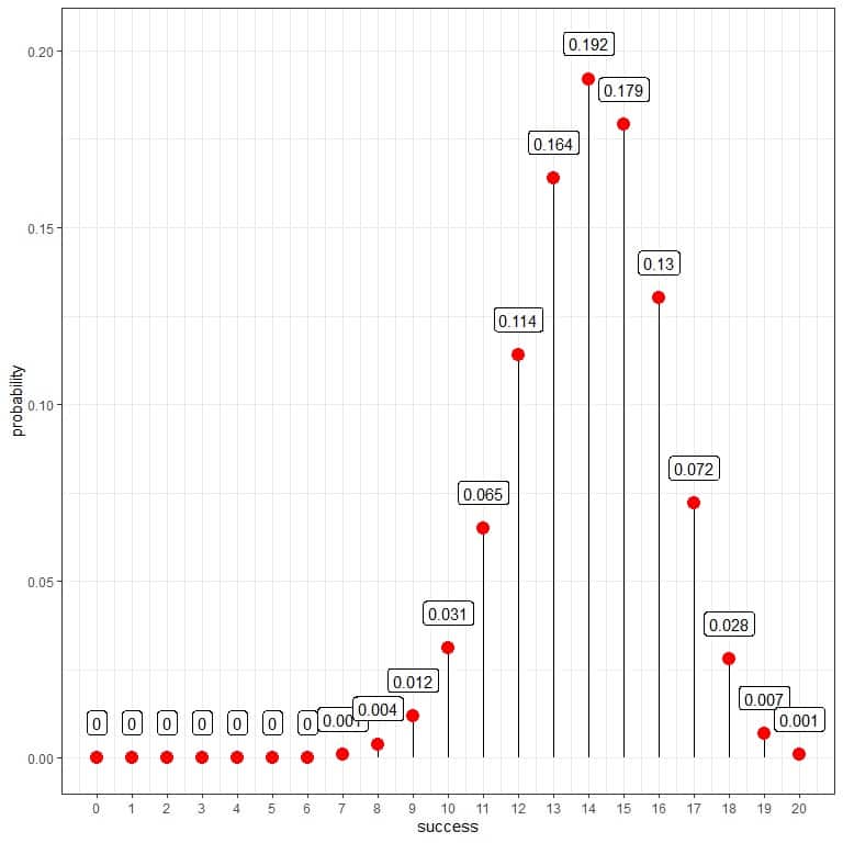
As the probability of success is 0.7, so the expected successes = 20 trials X 0.7 = 14.

We see that 14 (meaning that we found 14 heads and 7 tails from these 20 trials) has the highest probability. As we move away from 14, the probability fades away.

and as a curve:

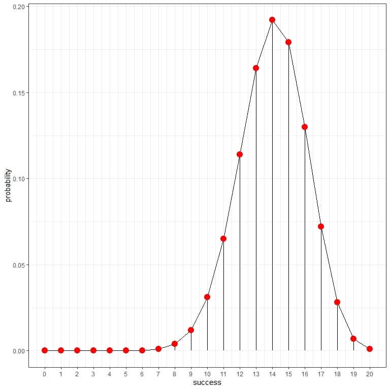
Here the probability of 5 heads in 20 trials of this unfair coin is almost zero.

Example 4

The prevalence of a particular disease in the general population is 10%. If you randomly select 100 persons from this population, what probability will you find all these 100 persons have the disease?

This is a binomial random process because:

1. Only 100 persons are randomly selected.
2. Each randomly selected person can be with only two possible outcomes (diseased or healthy). We call one of these outcomes (diseased) successful and the other (healthy) a failure.
3. The probability of a diseased person is the same in every person that is 10% or 0.1.
4. The persons are independent of each other because they are selected randomly from the population.

The number of persons with the disease in this sample can be:
0, 1, 2, 3, 4, 5, 6, ………….., or 100.

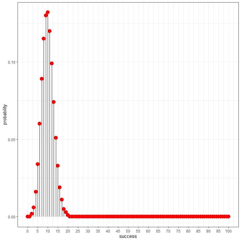
The binomial distribution can help us to calculate the probability of the total number of persons with diseasefound, and we get the following plot:

and as a curve:

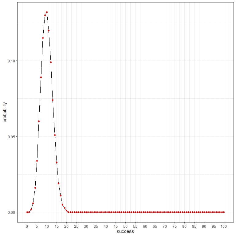
As the probability of a diseased person is 0.1, so the expected number of persons with diseasefound in this sample = 100 persons X 0.1 = 10.

We see that 10 (meaning that 10 persons with disease are in this sample and the remaining 90 are healthy) have the highest probability. As we move away from 10, the probability fades away.

The probability of 100 persons with disease in a sample of 100 is almost zero.

If we change the question and consider the number of healthy persons found, the probability of healthy person = 1-0.1 = 0.9 or 90%.

The binomial distribution can help us calculate the probability of the total number of healthy persons found in this sample. We get the following plot:

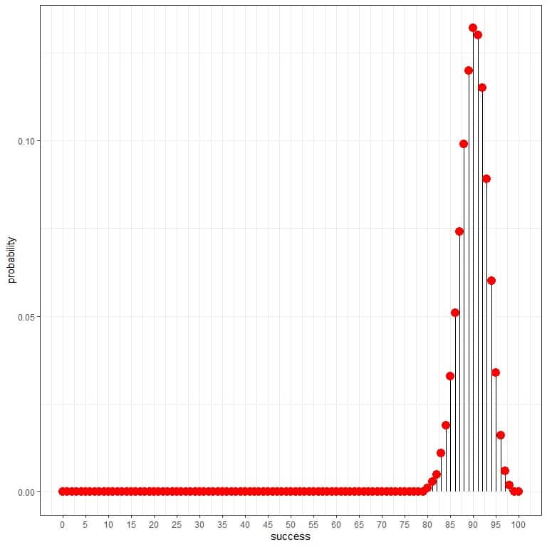
and as a curve:

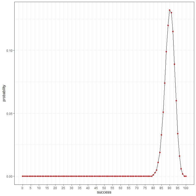
As the probability of healthy persons is 0.9, so the expected number of healthy persons found in this sample = 100 persons X 0.9 = 90.

We see that 90 (meaning 90 healthy persons we found in the sample and the remaining 10 are diseased) has the highest probability. As we move away from 90, the probability fades away.

Example 5

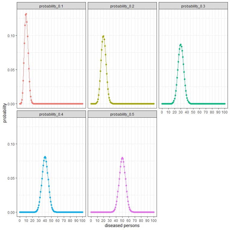
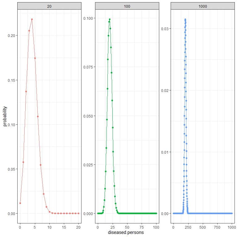
If the disease prevalence is 10%, 20%, 30%, 40%, or 50%, and 3 different research groups randomly select 20, 100, and 1000 persons respectively. What is the probability of the different number of persons with diseasefound?

For the research group that randomly selects 20 persons, the number of persons with disease in this sample can be 0, 1, 2, 3, 4, 5, 6, ….., or 20.

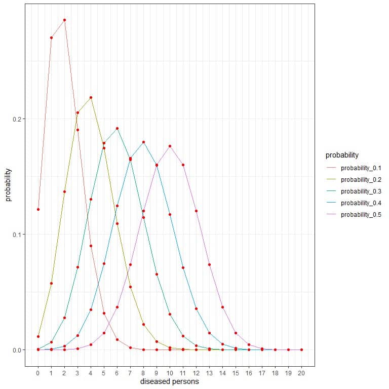
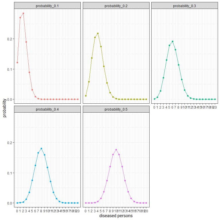
The different curves represent the probability of each number from 0 to 20 with different prevalence (or probabilities).

The peak of every curve represents the expected value,

When the prevalence is 10% or probability = 0.1, the expected value = 0.1 X 20 = 2.

When the prevalence is 20% or probability = 0.2, the expected value = 0.2 X 20 = 4.

When the prevalence is 30% or probability = 0.3, the expected value = 0.3 X 20 = 6.

When the prevalence is 40% or probability = 0.4, the expected value = 0.4 X 20 = 8.

When the prevalence is 50% or probability = 0.5, the expected value = 0.5 X 20 = 10.

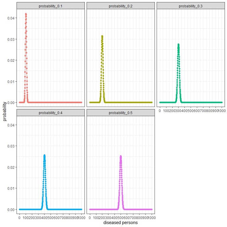
For the research group that randomly selects 100 persons, the number of persons with disease in this sample can be 0, 1, 2, 3, 4, 5, 6, ….., or 100.

The different curves represent the probability of each number from 0 to 100 with different prevalence (or probabilities).

The peak of every curve represents the expected value,
For prevalence 10% or probability = 0.1, the expected value = 0.1 X 100 = 10.

For prevalence 20% or probability = 0.2, the expected value= 0.2 X 100 = 20.

For prevalence 30% or probability = 0.3, the expected value = 0.3 X 100 = 30.

For prevalence 40% or probability = 0.4, the expected value = 0.4 X 100 = 40.

For prevalence 50% or probability = 0.5, the expected value = 0.5 X 100 = 50.

For the research group that randomly selects 1000 persons, the number of persons with disease in this sample can be 0, 1, 2, 3, 4, 5, 6, ….., or 1000.

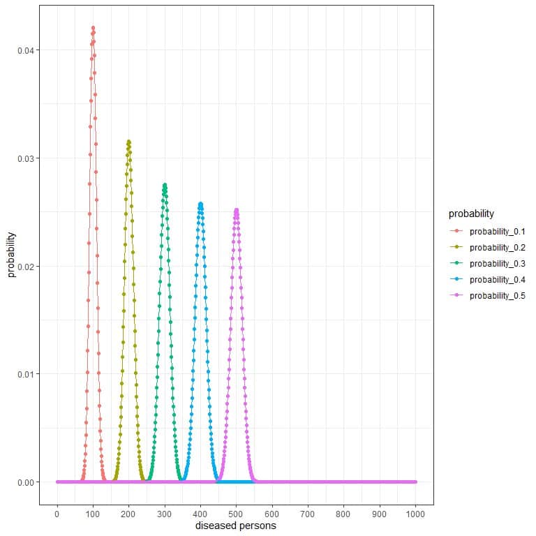
The x-axis represents the different number of persons with disease that may be found, from 0 to 1000.

The y-axis represents the probability for each number.

The peak of every curve represents the expected value,

For probability = 0.1, the expected value = 0.1 X 1000 = 100.

For probability = 0.2, the expected value = 0.2 X 1000 = 200.

For probability = 0.3, the expected value = 0.3 X 1000 = 300.

For probability = 0.4, the expected value = 0.4 X 1000 = 400.

For probability = 0.5, the expected value = 0.5 X 1000 = 500.

Example 6

For the previous example, if we want to compare the probability at different sample sizes and constant disease prevalence, which is 20% or 0.2.

The probability curve for 20 sample size will extend from 0 persons with the disease to 20 persons.

The probability curve for 100 sample size will extend from 0 persons with the diseaseto 100 persons.

The probability curve for 1000 sample size will extend from 0 persons with the disease to 1000 persons.

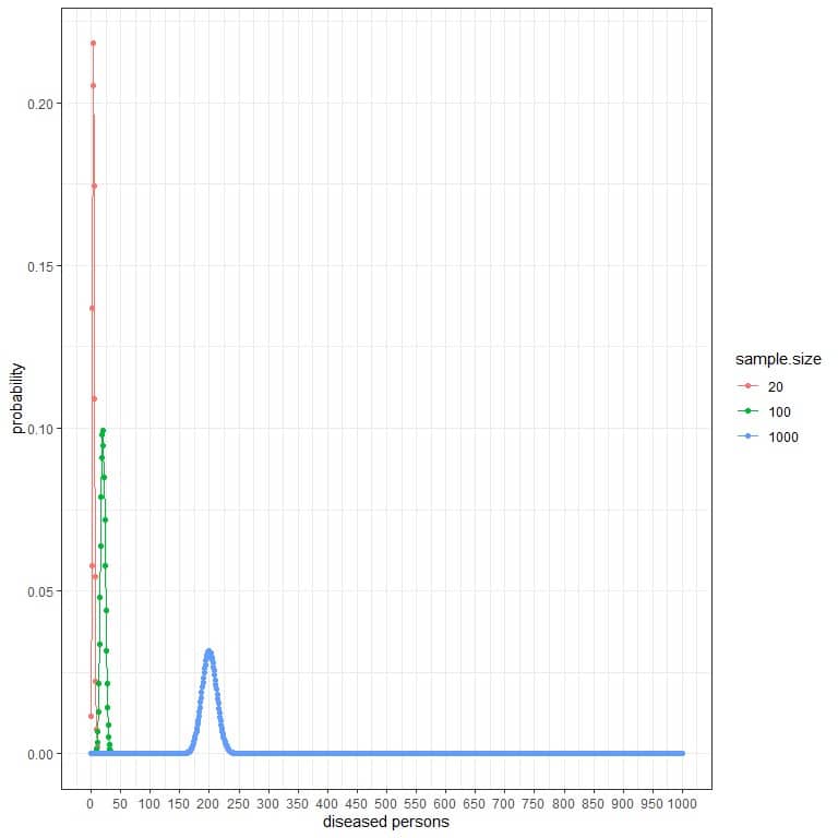
The peak or expected value for 20 sample size is at 4, while the peak for 100 sample size is at 20, and the peak for 1000 sample size is at 200.

Binomial distribution formula

If the random variable X follows the binomial distribution with n trials and the probability of success p, the probability of getting exactly k successes is given by:

f(k,n,p)=(n¦k) p^k (1-p)^(n-k)

where:

f(k,n,p) is the probability of k successes in n trials with probability of success, p.

(n¦k)=n!/(k!(n-k)!) and n! = n X n-1 X n-2 X….X 1. This is called factorial n. 0! = 1.

p is the probability of success, and 1-p is the probability of failure.

How to do binomial distribution?

To calculate the binomial distribution for the different number of successes, we only need the number of trials (n) and the probability of success (p).

Example 1

For a fair coin, what is the probability of 2 heads in 2 tosses?

This is a binomial random process with only two outcomes, head or tail. As it is a fair coin, so the probability of head (or success) = 50% or 0.5.

1. Number of trials (n) = 2.
2. The probability of head (p) = 50% or 0.5.
3. The number of successes (k) = 2.
4. n!/(k!(n-k)!) = 2 X 1/(2X 1 X (2-2)!) = 2/2 = 1.
5. n!/(k!(n-k)!) p^k (1-p)^(n-k) = 1 X 0.5^2 X 0.5^0 = 0.25.

The probability of 2 heads in 2 tosses is 0.25 or 25%.

Example 2

For a fair coin, what is the probability of 3 heads in 10 tosses?

This is a binomial random process with only two outcomes, head or tail. As it is a fair coin, so the probability of head (or success) = 50% or 0.5.

1. Number of trials (n) = 10.
2. The probability of head (p) = 50% or 0.5.
3. The number of successes (k) = 3.
4. n!/(k!(n-k)!) = 10X9X8X7X6X5X4X3X2X1/(3X2X1 X (10-3)!) = 10X9X8X7X6X5X4X3X2X1/((3X2X1) X (7X6X5X4X3X2X1)) = 120.
5. n!/(k!(n-k)!) p^k (1-p)^(n-k) = 120 X 0.5^3 X 0.5^7 = 0.117.

The probability of 3 heads in 10 tosses is 0.117 or 11.7%.

Example 3

If you rolled a fair die 5 times, what is the probability of getting 1 six, 2 sixes, or 5 sixes?

This is a binomial random process with only two outcomes, getting six or not. Since it is a fair die, the probability of six (or success) = 1/6 or 0.17.

To calculate the probability of 1 six:

1. Number of trials (n) = 5.
2. The probability of six (p) = 0.17. 1-p = 0.83.
3. The number of successes (k) = 1.
4. n!/(k!(n-k)!) = 5X4X3X2X1/(1 X (5-1)!) = 5X4X3X2X1/(1 X 4X3X2X1) = 5.
5. n!/(k!(n-k)!) p^k (1-p)^(n-k) = 5 X 0.17^1 X 0.83^4 = 0.403.

The probability of 1 six in 5 rollings is 0.403 or 40.3%.

To calculate the probability of 2 sixes:

1. Number of trials (n) = 5.
2. The probability of six (p) = 0.17. 1-p = 0.83.
3. The number of successes (k) = 2.
4. n!/(k!(n-k)!) = 5X4X3X2X1/(2X1 X (5-2)!) = 5X4X3X2X1/(2X1 X 3X2X1) = 10.
5. n!/(k!(n-k)!) p^k (1-p)^(n-k) = 10 X 0.17^2 X 0.83^3 = 0.165.

The probability of 2 six in 5 rollings is 0.165 or 16.5%.

To calculate the probability of 5 sixes:

1. Number of trials (n) = 5.
2. The probability of six (p) = 0.17. 1-p = 0.83.
3. The number of successes (k) = 5.
4. n!/(k!(n-k)!) = 5X4X3X2X1/(5X4X3X2X1 X (5-5)!) = 1.
5. n!/(k!(n-k)!) p^k (1-p)^(n-k) = 1 X 0.17^5 X 0.83^0 = 0.00014.

The probability of 5 sixes in 5 rollings is 0.00014 or 0.014%.

Example 4

The average rejection percentage for chairs from a particular factory is 12%. What is the probability that from a random batch of 100 chairs, we will found:

1. No rejected chairs.
2. Not more than 3 rejected chairs.
3. At least 5 rejected chairs.

This is a binomial random process with only two outcomes, rejected or good chair. The probability of rejected chair = 12% or 0.12.

To calculate the probability of No rejected chairs:

1. Number of trials (n) = sample size = 100.
2. The probability of rejected chair (p) = 0.12. 1-p = 0.88.
3. The number of successes or number of rejected chairs (k) = 0.
4. n!/(k!(n-k)!) = 100X99X…X2X1/(0! X (100-0)!) = 1.
5. n!/(k!(n-k)!) p^k (1-p)^(n-k) = 1 X 0.12^0 X 0.88^100 = 0.000002.

The probability of no rejections in a batch of 100 chairs = 0.000002 or 0.0002%.

To calculate the probability of not more than 3 rejected chairs:

The probability of not more than 3 rejected chairs = the probability of 0 rejected chairs + probability of 1 rejected chair + probability of 2 rejected chairs + probability of 3 rejected chairs.

1. Number of trials (n) = sample size = 100.
2. The probability of rejected chair (p) = 0.12. 1-p = 0.88.
3. The number of successes or number of rejected chairs (k) = 0,1,2,3.

We will calculate the factorial part, n!/(k!(n-k)!), p^k, and (1-p)^(n-k) separately for each number of rejections.

Then probability = “factorial part” X “p^k” X “(1-p)^{n-k}”.

We sum these probabilities to get the probability of not more than 3 rejected chairs.

0.00000280716+0.00003827946+0.00025838635+0.00115099373 = 0.00145.

The probability of not more than 3 rejected chairs in a batch of 100 chairs = 0.00145 or 0.145%.

To calculate the probability of at least 5 rejected chairs:

The probability of at least 5 rejected chairs = the probability of 5 rejected chairs + probability of 6 rejected chairs + probability of 7 rejected chairs +………+ probability of 100 rejected chairs.

Instead of calculating the probability for these 96 numbers (from 5 to 100), we can calculate the numbers’ probability from 0 to 4. Then, we sum these probabilities and subtract that from 1.

This is because the sum of probabilities is always 1.

1. Number of trials (n) = sample size = 100.
2. The probability of rejected chair (p) = 0.12. 1-p = 0.88.
3. The number of successes or number of rejected chairs (k) = 0,1,2,3,4.

We will calculate the factorial part, n!/(k!(n-k)!), p^k, and (1-p)^(n-k) separately for each number of rejections.

Then probability = “factorial part” X “p^k” X “(1-p)^{n-k}”.

We sum these probabilities to get the probability of not more than 4 rejected chairs.

0.00000280716+0.00003827946+0.00025838635+0.00115099373+ 0.00380612698 = 0.0053.

The probability of not more than 4 rejected chairs in a batch of 100 chairs = 0.0053 or 0.53%.

The probability of at least 5 rejected chairs = 1-0.0053 = 0.9947 or 99.47%.

Practice questions

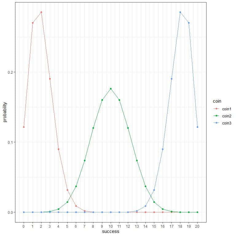
1. We have 3 probability distributions for 3 types of coins tossed 20 times.

Which coin is fair (meaning that probability of success or head = probability of failure or tail = 0.5)?

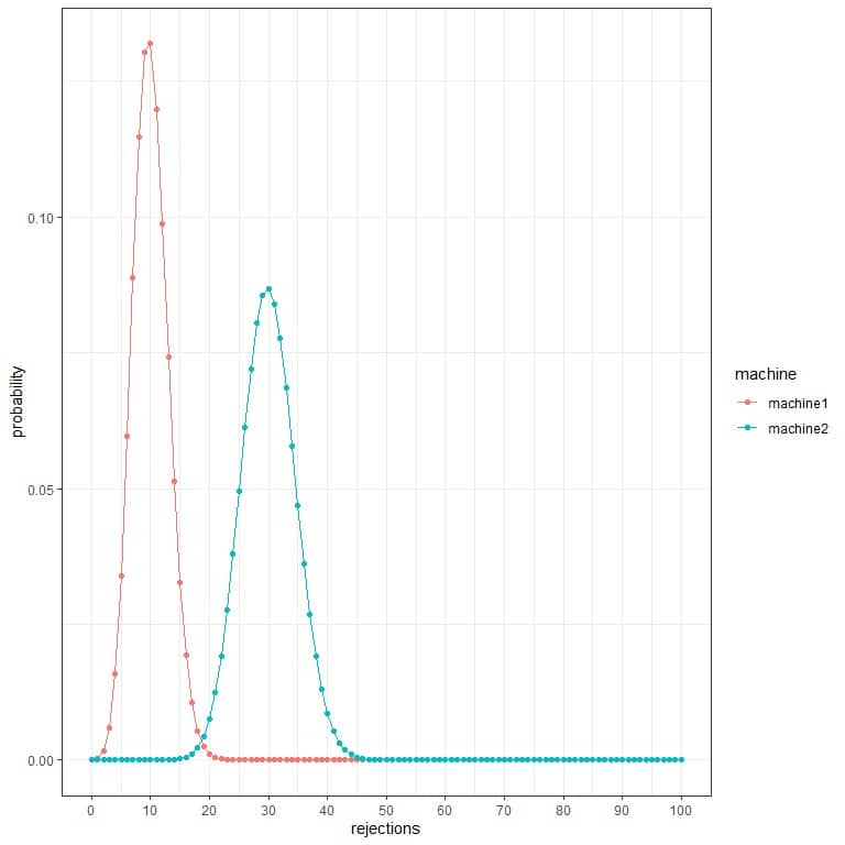
2. We have two machines for producing tablets in a pharmaceutical company. To test if the tablets’ are efficient, we need to take 100 different random samples from each machine. We also count the number of rejected tablets in every 100 random samples.

We use the number of rejected tablets to create different probability distribution for the number of rejections from each machine.

Which machine is better?

What is the expected number of rejected tablets from machine1 and machine2?

3. Clinical trials have shown that the effectiveness of one COVID-19 vaccine is 90%, and another vaccine has 95% effectiveness. What is the probability that both vaccines will cure the whole 100 COVID-19 infected patients of a random sample of 100 infected patients?

4. Clinical trials have shown that the effectiveness of one COVID-19 vaccine is 90%, and another vaccine has 95% effectiveness. What is the probability that both vaccines will cure at least 95 COVID-19 infected patients of a random sample of 100 infected patients?

5. As estimated by the World Health Organization (WHO), the probability of male births is 51%. For 100 births in a particular hospital, what is the probability that 50 births will be males and the other 50 will be females?

Answer key

1. We see that coin2 is a fair coin from the plot because the expected value (peak) = 20 X 0.5 = 10.

2. This is a binomial process because the outcome is either a rejected or good tablet.

Machine1 is better because its probability distribution is at lower values than that for machine2.

The expected number (peak) of rejected tablets from machine1 = 10.

The expected number (peak) of rejected tablets from machine2 = 30.

This also confirms that machine1 is better than machine2.

3. This is a binomial random process with only two outcomes, cured patient or not. The probability of curing = 90% for one vaccine and 95% for the other vaccine.

To calculate the probability of curing for the 90% effective vaccine:

• Number of trials (n) = sample size = 100.
• The probability of curing (p) = 0.9. 1-p = 0.1.
• The number of cured patients (k) = 100.
• n!/(k!(n-k)!) = 100X99X…X2X1/(100! X 0!) = 1.
• n!/(k!(n-k)!) p^k (1-p)^(n-k) = 1 X 0.9^100 X 0.1^0 = 0.0000265614.

The probability of curing all 100 patients = 0.0000265614 or 0.0027%.

To calculate the probability of curing for the 95% effective vaccine:

• Number of trials (n) = sample size = 100.
• The probability of curing (p) = 0.95. 1-p = 0.05.
• The number of cured patients (k) = 100.
• n!/(k!(n-k)!) = 100X99X…X2X1/(100! X 0!) = 1.
• n!/(k!(n-k)!) p^k (1-p)^(n-k) = 1 X 0.95^100 X 0.05^0 = 0.005920529.

The probability of curing all 100 patients = 0.005920529 or 0.59%.

4. This is a binomial random process with only two outcomes, cured patient or not. The probability of curing = 90% for one vaccine and 95% for the other vaccine.

To calculate the probability for the 90% effective vaccine:

The probability of at least 95 cured patients in a sample of 100 patients = the probability of 100 cured patients + probability of 99 cured patients + probability of 98 cured patients + probability of 97 cured patients + probability of 96 cured patients + probability of 95 cured patients.

• Number of trials (n) = sample size = 100.
• The probability of curing (p) = 0.9. 1-p = 0.1.
• The number of successes or number of cured patients (k) = 100,99,98,97,96,95.

We will calculate the factorial part, n!/(k!(n-k)!), p^k, and (1-p)^(n-k) separately for each number of cured patients.

Then probability = “factorial part” X “p^k” X “(1-p)^{n-k}”.

We sum these probabilities to get the probability of at least 95 cured patients.

0.0000265614+ 0.0002951267+ 0.0016231966+ 0.0058916025+ 0.0158745955+ 0.0338658038 = 0.058.

The probability of at least 95 cured patients in a sample of 100 patients = 0.058 or 5.8%.

Consequently, the probability of not more than 94 cured patients = 1-0.058 = 0.942 or 94.2%.

To calculate the probability for the 95% effective vaccine:

• Number of trials (n) = sample size = 100.
• The probability of curing (p) = 0.95. 1-p = 0.05.
• The number of successes or number of cured patients (k) = 100,99,98,97,96,95.

We will calculate the factorial part, n!/(k!(n-k)!), p^k, and (1-p)^(n-k) separately for each number of cured patients.

Then probability = “factorial part” X “p^k” X “(1-p)^{n-k}”.

We sum these probabilities to get the probability of at least 95 cured patients.

0.005920529+ 0.031160680+ 0.081181772+ 0.139575678+ 0.178142642+ 0.180017827 = 0.616.

The probability of at least 95 cured patients in a sample of 100 patients = 0.616 or 61.6%.

Consequently, the probability of not more than 94 cured patients = 1-0.616 = 0.384 or 38.4%.

5. This is a binomial random process with only two outcomes, male birth or female birth. The probability of male birth = 51%.

To calculate the probability of 50 male births:

• Number of trials (n) = sample size = 100.
• The probability of male birth (p) = 0.51. 1-p = 0.49.
• The number of male births (k) = 50.
• n!/(k!(n-k)!) = 100X99X…X2X1/(50! X 50!) = 1 X 10^29.
• n!/(k!(n-k)!) p^k (1-p)^(n-k) = 1 X 10^29 X 0.51^50 X 0.49^50 = 0.077.

The probability of exactly 50 male births in 100 births = 0.077 or 7.7%.

Previous Lesson | Main Page | Next Lesson