Green’s theorem – Theorem, Applications, and Examples

Green’s Theorem is one of the most important theorems that you’ll learn in vector calculus.  This theorem helps us understand how line and surface integrals relate to each other. When a line integral is challenging to evaluate, Green’s theorem allows us to rewrite to a form that is easier to evaluate.

Green’s Theorem allows us to connect our understanding of line integrals and integration of multivariable functions. Through Green’s theorem, we can rewrite line integrals in terms of double integrals.

Our discussion will cover the fundamentals of Green’s theorem – from its definition to its proof. We’ll also cover the general form of Green’s theorem and its many applications. Before we proceed, make sure that you have a strong grasp on the following topics:

• Knowing how to evaluate iterated integrals.
• Understanding the second part of the fundamental theorem of calculus.
• Being familiar with the process of evaluating line integrals and knowing how to apply the fundamental theorem for the line integral.

For now, let’s break down the important components of Green’s theorem and understand the theorem’s definition.

What Is Green’s Theorem?

Green’s theorem allows us to integrate regions that are formed by a combination of a line and a plane. It allows us to find the relationship between the line integral and double integral – this is why Green’s theorem is one of the four core concepts of the fundamental theorem of Calculus.

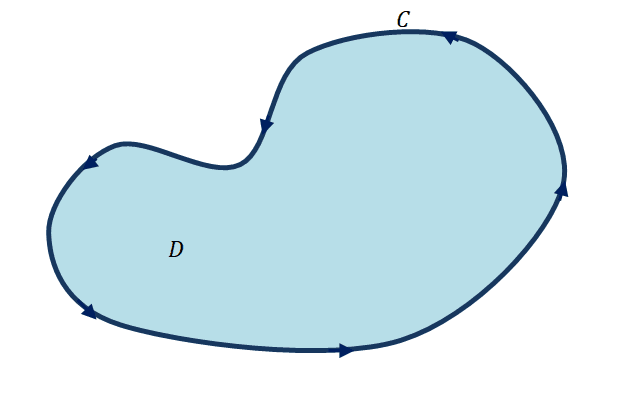
Before we discuss the formula for Green’s theorem, let’s go first to take a look at the curve shown above. The graph above highlights a closed curve defined by $C$ and the enclosed region is labeled as the region, $D$. The curve, $C$, is going around in a counterclockwise direction. Throughout our discussion, for consistency, we consider the curve positively oriented when it follows a counterclockwise direction. This also means that when the path of the curve is in a clockwise direction is negatively oriented. The curve shown is also simple because it goes through the path with no loops while the region is considered simply connected because it encloses no holes.

It is important that we know these terms and some properties of curves before establishing Green’s theorem.

Green’s Theorem Formula

Suppose that $C$ is a simple, piecewise smooth, and positively oriented curve lying in a plane, $D$, enclosed by the curve, $C$. When $M$ and $N$ are two functions defined by $(x, y)$ within the enclosed region, $D$, and  the two functions have continuous partial derivatives, Green’s theorem states that:

\begin{aligned}\oint_{C} \textbf{F} \cdot d\textbf{r}&= \oint_{C} M \phantom{x}dx + N \phantom{x}dy\\ &= \int \int_{D} \left(\dfrac{\partial N}{\partial x} -\dfrac{\partial M}{\partial y}\right ) \phantom{x}dx \phantom{x}dy  \end{aligned}

Keep in mind that the symbol, $\oint_{C}$, represents the integral of the function over the curve, $C$. We use this symbol when we want to highlight that the curve, $C$, is a closed curve in positive orientation. When you also see this symbol, this means that the curve meets the conditions of Green’s theorem.

Let’s now break down the formula representing the Green’s theorem. If we want to find the area of the simple curve that has a line integral,

\begin{aligned} \oint M \phantom{x}dx + N \phantom{x}dy,\end{aligned}

we can rewrite the line integral as a double integral using the partial derivatives of $M$ and $N$:

\begin{aligned} \int \int_{D} \left(\dfrac{\partial N}{\partial x} -\dfrac{\partial M}{\partial y}\right ) \phantom{x}dA \end{aligned}

Now that we’ve established Green’s theorem, it’s time that we know how to prove and apply the formula for Green’s theorem. Let’s start with its proof and then the next two sections will cover its application.

Green’s Theorem Proof

The proof of Green’s theorem has three phases: 1) proving that it applies to curves where the limits are from $x = a$ to $x=b$, 2) proving it for curves bounded by $y=c$ and $y = d$, and 3) accounting for curves made up of that meet these two forms.

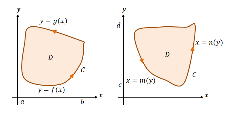
These are examples of the first two regions we need to account for when proving Green’s theorem. The first region shows a curve a enclosing it defined by $y= f(x)$ and $y = g(x)$ and bounded from $x =a$ to $x =b$. At the straight vertical edges, we can conclude that $dx = 0$. We can write the line integral for the region as shown below.

\begin{aligned} \oint_{C} M(x, y)\phantom{x} dx &= \int_{a}^{b} M(x, f(x)) \phantom{x}dx + \int_{b}^{a} M(x, g(x)) \phantom{x}dx \\&= \int_{a}^{b} [M(x, f(x)) – M(x, g(x))]\phantom{x} dx\end{aligned}

Let’s now write the double integral to show how we can relate the line and double integrals of the region.

\begin{aligned} \int \int_{D} M_y \phantom{x} dA &= \int_{a}^{b} \int_{f(x)}^{g(x)} M_y(x, y) \phantom{x}dydx\\&= \int_{a}^{b} [M(x, g(x)) – M(x,f(x))]\phantom{x} dx\\&= -\oint_{C} M(x, y)\phantom{x}dx \end{aligned}

From this, we’ve confirmed the first phase: showing that $\oint M(x, y)\ phantom{x}dx = – \int \int_{D} M_y \phantom{x}dA$. Apply a similar approach to work on the second phase.

\begin{aligned}\oint_{C} N(x, y)\phantom{x} dy &= \int_{d}^{c} N(m(y), y) \phantom{x}dy +\int_{c}^{d} N(n(y), y) \phantom{x}dy \\&= \int_{c}^{d} [N(n(y), y) – N(m(y), y)]\phantom{x} dy\\&= \int_{c}^{d} \int_{m(y)}^{n(y)} N_x(x, y) \phantom{x} dxdy\\&= \int\int_{D} N_x \phantom{x}dA\end{aligned}

Now, let’s move on to the third phase: combining these two phases to account for regions defined by a combination of these curve types.

\begin{aligned}\oint_{C} M(x,y) \phantom{x}dx + N(x, y)\phantom{x} dy &= \int\int_{D} (N_x – M_y) \phantom{x}dA\\&= \int\int_{D} \left(\dfrac{\partial N}{\partial x}- \dfrac{\partial M}{\partial y}\right) \phantom{x}dA\end{aligned}

Even when we work with regions enclosed by several curves, the theorem still applies since we’ll simply combine all curves of each type. This concludes our proof for Green’s theorem. It’s time that we learn how to apply the formula properly.

How To Use Green’s Theorem?

We can use Green’s theorem by taking the partial derivatives of the two or more curves that define the enclosed region. Go through this guideline to help you apply Green’s theorem formula:

1. Identify the components of the vector fields: $M(x, y)$ and $N(x, y)$.
2. Confirm that the curve, $C$, satisfies the conditions needed for us to apply Green’s theorem.
3. Find expressions for $\dfrac{\partial M}{\partial y}$ and $\dfrac{\partial N}{\partial x}$ then take their difference: $\left(\dfrac{\partial N}{\partial x} – \dfrac{\partial M}{\partial y}\right)$.
4. Assign appropriate limits of integration then evaluate the double integral $\int \int_{D} \left(\dfrac{\partial N}{\partial x} – \dfrac{\partial M}{\partial y}\right) \phantom{x}dA$.

Let’s try to calculate the line integral, $\oint_{C} xy^2 \phantom{x}dx + (y – 4) \phantom{x}dy$, where $C$ is defined the rectangle with the following vertices: $(1, -1)$, $(4, -1)$, $(4, 2)$, and $(1, 2)$ and the rectangle is positively oriented.

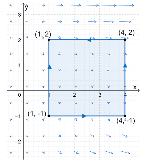
Here’s the graph of the curve, $C$, lying on the vector field, $\textbf{F}(x, y) = <M(x, y), N(x, y)> = <x^2y, y – 4>$. This means that $M(x, y) = x^2y$ and $N(x, y) = y – 4$.

We can also confirm that $C$ is a simple, smooth, and closed plane. Since it’s also given that it is oriented in the counterclockwise direction, we have shown that we can apply the Green’s theorem to evaluate the line integral. Let’s now find the partial derivative of $M(x, y)$ with respect to $y$ and the partial derivative of $N(x,y )$ with respect to $x$.

Using these expressions, we have $\dfrac{\partial N}{\partial x} – \dfrac{\partial M}{\partial y} = -x^2$. Let’s now use the Green’s theorem to evaluate $\oint_{C} \textbf{F} \cdot d\textbf{r}$, where the limits of integration for $x$ is $[1, 4]$ while for $y$, we have $[-1, 2]$.

\begin{aligned}\oint_{C} \textbf{F} \cdot d\textbf{r}&= \int \int_{D} \left(\dfrac{\partial N}{\partial x} -\dfrac{\partial M}{\partial y}\right ) \phantom{x}dx \phantom{x}dy\\&= \int_{-1}^{2} \int_{1}^{4} (-x^2) \phantom{x} dxdy\\&= \int_{-1}^{2}\left[-\dfrac{x^3}{3} \right ]_{1}^{4} \phantom{x}dy\\&= \int_{-1}^{2} -21\phantom{x}dy\\&= [-21y]_{-1}^{2}\\&= -21(2- – 1) \\&= -63 \end{aligned}

This shows how we can evaluate line integrals using Green’s theorem. Noticed how we didn’t have to parametrize the vector field first? This reduces the time spent to evaluate the line integral – especially when they satisfy the conditions for Green’s theorem.

Now that we’ve shown you how to utilize it, it’s time for us to explore the times when Green’s theorem is the most useful.

When To Use Green’s Theorem?

We can use Green’s theorem when we’re given complex expressions for the curves of complex line integrals.  Here are some more instances when Green’s theorem is extremely helpful:

• They come in handy when we have to break down the line integral into line integrals with shorter paths.
• We can use Green’s theorem when evaluating line integrals of the form, $\oint M(x, y) \phantom{x}dx + N(x, y) \phantom{x}dy$, on a vector field function.
• This theorem is also helpful when we want to calculate the area of conics using a line integral.
• We can apply Green’s theorem to calculate the amount of work done on a force field.
• We can also calculate flux and water flow using Green’s theorem.

Here’s an important reminder though: review if the curve, $C$, satisfies the

For example, we can use Green’s theorem if we want to calculate the work done on a particle if the force field is equal to $\textbf{F}(x, y) = <y – \cos x, e^y – 2x>$. Suppose that the particle travels around the curve represented by the equation, $x^2 + y^2 = 9$, in a counterclockwise direction. The particle starts and ends at the point, $(3, 0)$.

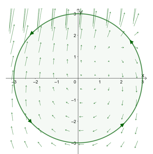
The graph above illustrates the motion of the particle on the force field. Since the curve, $C$, is a smooth and closed circle that is positively oriented, we can apply the Green’s theorem to calculate the work done on the particle.

\begin{aligned}\text{Work} &= \oint_{C} \textbf{F} \cdot d\textbf{r}\end{aligned}

We’ve learned how to calculate work using the fundamental theorem for line integral, so let’s show you how we can calculate work done when the path is a circular curve. We have $\textbf{F}(x, y) = <y – \cos x, e^y – 2x>$, so we can rewrite the line integral representing work as shown below.

\begin{aligned}\text{Work} &= \oint M(x, y) \phantom{x}dx + N(x, y) \phantom{x}dy\\&= \oint (y – \cos x) \phantom{x}dx + (e^y – 2x) \phantom{x}dy\end{aligned}

Let’s now take the partial derivatives of $

This means that $\dfrac{\partial N}{\partial x} – \dfrac{\partial M}{\partial y}$ is equal to $-3$. We just need to evaluate the double integral of $-3$ to find the total amount of work done on the particle – this is all thanks to Green’s theorem. From the graph, we can see that our limits of integration are from $-2$ to $2$ for both $x$ and $y$. We also know that the area of $D$ is equal to $\pi(3^2) = 9\pi$ squared units.

\begin{aligned}\text{Work} &= \int \int -3 \phantom{x}dA\\&= (\text{Area}_D)(9\pi)\\&= -3(9\pi)\\&= -27\pi\end{aligned}

From this, we can see that the total amount of work done on the particle is equal to $-27\pi$ units.  We’ve shown you the benefits of understanding this core theorem, so this time, test your understanding and master this topic further by trying out the examples shown below.

Example 1

Evaluate the line integral, $\oint_{C} y^3 \phantom{x}dx – x^3 \phantom{x}dy$, where $C$ is the curve defined by the equation, $x^2 + y^2  = 4$. The curve is formed starting from $(-2, 0)$ and is positively oriented.

Solution

We’re given the vector field, $\textbf{F} = <y^3, -x^3>$, so we have $M(x, y) = y^3$ and $N(x, y) = -x^3$. Since $C$ is a circle centered at the origin with a radius of $2$ units, as shown below, the curve is simple, closed, and positively oriented.

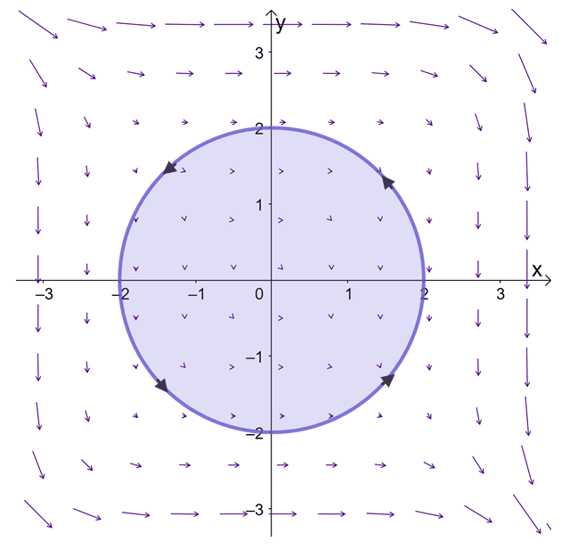
This means that we can use the Green’s thereom to evaluate $\oint_{C} y^3 \phantom{x}dx – x^3 \phantom{x}dy$. Let’s go ahead and find the partial derivatives of $y^3$ with respect to $y$ and $-x^3$ with respect to $x$.

Taking the difference between the two, we have $\dfrac{\partial N}{\partial x} – \dfrac{\partial M}{\partial y} = -3x^2 – 3y^2$. Now, let’s work on the double integral of this expression knowing that the enclosed region is a circle, so the polar limits of integration are $0 \leq r\leq 2$ and $0 \leq \theta \leq 2\pi$. Hence, we have the double integral shown below.

\begin{aligned}\oint_{C} y^3 \phantom{x}dx – x^3 \phantom{x}dy &= \int \int_{D} -3\left(x^2 + y^2 \right ) \\&= \int_{0}^{2\pi} \int_{0}^{2} -3r^2 \phantom{x}rdrd\theta\\&=-3\int_{0}^{2\pi} \int_{0}^{2} r^3 \phantom{x}drd\theta\\&=-3\int_{0}^{2\pi} \left[\dfrac{r^4}{4} \right ]_{0}^{2} \phantom{x}d\theta\\\\&=-3\int_{0}^{2\pi} 4 \phantom{x}d\theta\\&= -12[\theta]_{0}^{2\pi}\\&= -24\pi\end{aligned}

This means that $\oint_{C} y^3 \phantom{x}dx – x^3 \phantom{x}dy$ is equal to $-24\pi$.

Example 2

In the past, we’ve defined flux as the rate of fluids or energy over a given curve in a vector field. Mathematically, we can calculate it by taking the line integral of the vector field over the given curve: $\oint_{C} \textbf{F} \cdot \textbf{N} = \oint_{C} –N(x, y)\phantom{x} dx + M(x, y) \phantom{x}dy$.

Use this information to calculate the flux of $\textbf{F}(x, y) = <x^2  + e^y, 3x+ y>$ across the curve, $C$, where $C$ is a triangle with the following vertices: $(0, 0)$, $(2, 0)$, and $(0, 4)$.

Solution

We can write the flux of the vector field as $\oint_{C} \textbf{F} \cdot \textbf{N} phantom{x}ds$, where $C$ is defined by curves like the one we’re given.

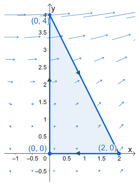
The triangle is in a clockwise direction, so at first glance, we may think that Green’s theorem won’t be applicable for this curve. Here’s an important property to remember about fluxes and closed curves: $\oint_{C} \textbf{F} \cdot \textbf{N} \phantom{x}ds=-\oint_{-C} \textbf{F} \cdot \textbf{N} \phantom{x}ds $. The curve, $-C$, represents the same figure, but this time, the curve is moving in a counterclockwise direction – meeting the conditions for Green’s theorem.

\begin{aligned}\oint_{C} \textbf{F} \cdot \textbf{N} \phantom{x}ds&=-\oint_{-C} \textbf{F} \cdot \textbf{N} \phantom{x}ds\\&= -\oint_C -(3x +y) \phantom{x}dx + (x^2 + e^y)\phantom{x}dy \end{aligned}

Let’s now evaluate the line integral by rewriting the expression as a double integral and applying the Green’s theorem. Keep in mind that this time, we have $M(x, y) = -(3x +y) $ and $N(x, y)= (x^2 + e^y)$, so $\dfrac{\partial N}{\partial x} = 2x$ and $\dfrac{\partial M}{\partial y} = -1$ and $\left(\dfrac{\partial N}{\partial x} – \dfrac{\partial M}{\partial y}\right) = (2x + 1)$.

\begin{aligned}\oint_{C} \textbf{F} \cdot \textbf{N} \phantom{x}ds &= -\int \int_{D} (2x + 1) \phantom{x} dA\end{aligned}

Let’s now work on the limits of integration, vertically, we can see that $y$ bounded from $y = 0$ to $y = -2x + 4$. Meanwhile, $x$ ranges from $x = 0$ to $x = 2$.

\begin{aligned} -\int \int_{D} (2x + 1) \phantom{x} dA &= – \int_{0}^{2} \int_{0}^{-2x + 4} (2x + 1) \phantom{x}dydx\\&= -\int_{0}^{2} (2x + 1)(-2x + 4) dx\\&= -\int_{0}^{2} -(4x^2 – 6x – 4) \phantom{x}dx\\&= \left[\dfrac{4x^3}{3} – \dfrac{6x^2}{2} – 4x\right ]_{0}^{2}\\&= -\dfrac{28}{3}\end{aligned}

This shows that the flux of the vector field is equal to $-\dfrac{28}{3}$ units.

Practice Questions

1. Evaluate the line integral, $\oint_{C} xy \phantom{x}dx + (x +y) \phantom{x}dy$, where $C$ is the curve defined by the equation, $x^2 + y^2 = 1$. The curve is formed starting from $(-1, 0)$ and is positively oriented.
2. Evaluate the line integral, $\oint_{C}e^{x^2} + y \phantom{x}dx + e^{2x} – y \phantom{x}dy$, where $C$ is the curve defined by the equation, $y = -(x^2 – 1)$. The curve is formed starting from $(1, 0)$ and is negatively oriented.
3. Calculate the flux of $\textbf{F}(x, y) = <x, y>$ across the curve, $C$, where $C$ is a circle defined by the equation, $x^2 + y^2 = 25$.
4. Calculate the flux of $\textbf{F}(x, y) = <2xy + 2x, -(y^2 – y – x)>$ across the curve, $C$, where $C$ is a circle defined by the equation, $x^2 + y^2 = 9$.

Answer Key

1. $\oint_{C} xy \phantom{x}dx + (x +y) \phantom{x}dy = \int_{0}^{2\pi} \int_{0}^{1} (1 – r\cos \theta)\phantom{x} rdrd\theta = \pi$
2. $\oint_{C} xy \phantom{x}dx + (x +y) \phantom{x}dy = -\int_{-1}^{1} \int_{0}^{1 – x^2} (1 – 2e^{2x}) \phantom{x}dydx =\dfrac{4}{2} – \dfrac{e^2}{2} – \dfrac{3}{2e^2}$
3. $\oint \textbf{F} \cdot \textbf{N} \phantom{x}ds = 50\pi$
4. $\oint \textbf{F} \cdot \textbf{N} \phantom{x}ds = 27\pi$

Images/mathematical drawings are created with GeoGebra.