JUMP TO TOPIC
Horizontal Compression – Properties, Graph, & Examples
 Is it possible for us to shrink or compress graphs horizontally? When do we compress graphs along the x-axis, and how does it affect its expression? These are some of the questions you’ll be able to answer once we learn about this unique transformation technique: horizontal compression.
Horizontal compressions occur when the function’s base graph is shrunk along the x-axis and, consequent, away from the y-axis.
Isn’t it interesting that by inspecting coefficients, we can either stretch or compress a function’s graph? Mastering the different types of transformations will save us time and help us better understand functions and graphs.
This is why we’ve written about this topic extensively. Think you need a refresher in any of these topics below? Feel free to click the links!
- Identify and learn how common parent functions are graphed.
- Master vertical and horizontal translations
- Learn how you can vertically and horizontally stretch graphs.
- Observe how vertical compressions are applied to graphs here.
As for this article’s goal, why don’t we go ahead and learn more about horizontal compression?
What is a horizontal compression?
Given that y = f(x) is the function that we want to transform, f(x) will undergo a horizontal compression when the scale factor, a ( where a > 1), is multiplied to the input value or x for this case.
This means that when we multiply x by a scale factor greater than 1, we expect its graph to shrink by the same scale factor.
Why don’t we compress f(x) = x2 by scale factors of 2 and 4?
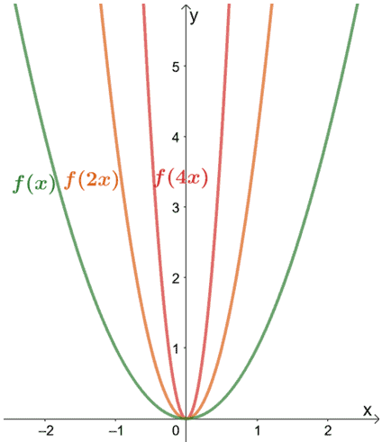
As can be observed from the graph, when we multiply x by 2, the new graph is a compressed version of the original graph. We also expect a similar effect when x is multiplied by 4, but this time, the graph compresses by a scale factor of 4.
Note that despite being compressed horizontally, the y-coordinates and intercepts remain the same. What do we expect from the transformed functions’ coordinates?
If the base function passes through (m, n), the horizontally compressed graph will pass through (m/a, n).
How to horizontally compress a function?
We’ve now seen how horizontal compressions affect the graph and points of a function’s graph. Why don’t we start applying our knowledge to compress and graph functions? Before we do, here are some important reminders to remember:
- Make sure to compress the base graph horizontally by checking the reference points’ new positions.
- The y-coordinates would remain in the same position. Consequently, make sure that the y-intercepts remain in the same position.
- Make sure that the graph and its points are scaled correctly.
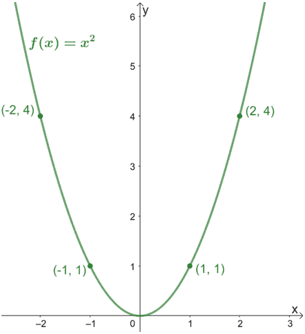
Why don’t we graph the parent function, f(x) = x2, and plot some reference points as well? Our goal is to graph the function g(x) = (4x)2.
Based on what we’ve just learned, make sure that the coordinate points’ x-coordinates are reduced by 1/4. The current points will now be:
- (-2, 4) → (-1/2, 4)
- (-1, 1) → (-1/4, 1)
- (1, 1) → (1/4, 1)
- (2, 4) → (1/2, 4)
Let’s go ahead and plot these points and the graph of g(x) to compare the two graphs.
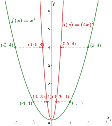
As we have expected, since g(x)’s input value is scaled by a factor of 4, we expect the graph of f(x) to shrink by the same scale factor.
The graph shown above confirms this and shows how g(x) is the result of f(x) being horizontally compressed by a scale factor of 4.
Summary of horizontal compression definition and properties
Are you ready to answer more problems involving horizontal compressions? Why don’t we recap what we learned so far first before we do:
- Horizontal compression depends on the scale factor multiplied by the input value (usually x).
- When f(x) is compressed horizontally to f(ax), divide the x-coordinates by a.
- Retain the y-intercepts and coordinates’ positions.
- The transformed function will have the same range but may have a different domain.
- When a function is compressed horizontally, its point transforms from (m, n) to (m/a, n).
When stuck on a problem or unsure what to do next when compressing a function horizontally, don’t hesitate to go back to these five pointers.
Let’s go ahead and try out problems that involve horizontal compression!
Example 1
Given that f(x) is equal to 12|x|, what is the expression for g(x) given that is the result of f(x) being compressed horizontally by a scale factor of 4?
a. g(x) = 3|x|
b. g(x) =4|x|
c. g(x) = 12|x|
d. g(x) =48|x|
Solution
When we compress a function horizontally, we multiply the input value by the scale factor. Hence, we have
g(x) = f( 4x)
= 12|4x|
= 48|x|
Example 2
Write the expressions for g(x) and h(x) in terms of f(x) given the following conditions:
a. When we horizontally compress f(x) by a scale factor of 4, we obtain g(x).
b. The function h(x) is the result of g(x) being compressed horizontally by a factor of 2.
Solution
Let’s first find the expression for g(x) in terms of f(x). Since, g(x) is the result of horizontally compressing f(x), we multiply the input value of f(x) by 4.
g(x) = f(2 ·x)
= f(2x)
Now that we have g(x) in terms of f(x), we can use this to find the expression for h(x).
h(x) = g(2x)
= f(2 ∙ 2x)
= f(4x)
Hence, we have g(x) = f(2x) and h(x) = f(4x).
Example 3
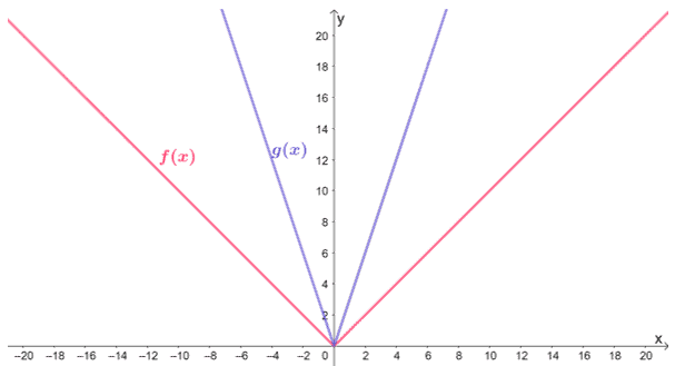
Determine the relationship shared by f(x) and g(x) based on the graphs shown below.
Solution
From the graph alone, we can see that g(x) is the result of f(x) being horizontally compressed. Let’s go ahead and note some reference points to find the scale factor needed to compress f(x) to g(x) horizontally.
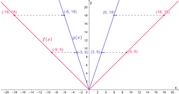
- (-18, 18) → (-6, 18)
- (-9, 9) → (-3, 9)
- (9, 9) → (3, 9)
- (18, 18) → (6, 18)
We can see that the input values decreased by 1/3, so the scale factor applied on f(x) is 3, and so, g(x) = f(3x).
This means that the function g(x) is the result of f(x) being horizontally compressed by a scale factor of 3.
Example 4
Apply what you know so far and describe the transformations performed for each pair of functions.
a. f(x) = x2 → g(x) = 16x2
b. m(x) = √x → n(x) = 2√(3x)
c. p(x) = |x| → q(x) = |2x| + 4
Solution
By reviewing each pair of graphs, we can see that some may require other transformations that we have learned from the past.
Let’s go ahead and start with the first pair, f(x) and g(x):
Express g(x) as a perfect square to determine the changes applied to f(x). We have g(x) = (4x)2. From this, we can see that g(x) is the result of f(x) being compressed horizontally by a scale factor of 4.
Moving on to m(x) and n(x):
From the two expressions, we can see that n(x) is the result if m(x) being scaled vertically and horizontally. Let’s inspect the coefficients and see what they represent:
n(x) = 2 ∙ m(3x)
We can see that n(x) is the result of m(x) being stretched vertically by a scale factor of 2 and compressed horizontally by a scale factor of 3.
Lastly, let’s see the transformations done on p(x) to reach q(x).
q(x) = p(2x) + 4
Hence, q(x) results from p(x) being compressed horizontally by a scale factor of 2 and translated 4 units downward.
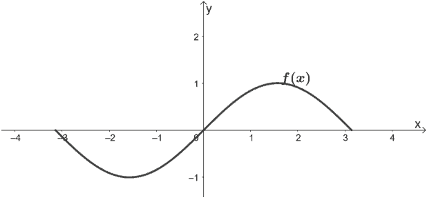
Example 5
What are the transformations done on f(x) = sin x so that it results to g(x) = 3 sin (2x) + 1? Use the graph of f(x) (from -π to π) shown below then apply the transformations to graph g(x).
Solution
First, let’s observe the transformations applied on f(x) to attain g(x).
g(x) = 3 ∙ sin (2 ∙ x) + 1
= 3 f(2x) + 1
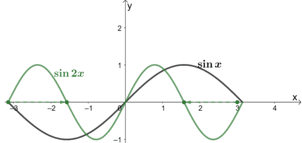
From this, we can see that to attain g(x), we need to compress f(x) horizontally by a factor of 2, vertically stretch f(x) by a scale factor of 3, and translate the resulting function 1 unit upward.
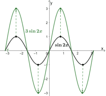
Let’s slowly graph g(x) by applying these transformations. Let’s start by horizontally compressing f(x) by a scale factor of 2.
Next, let’s vertically stretch the resulting function by a scale factor of 3.
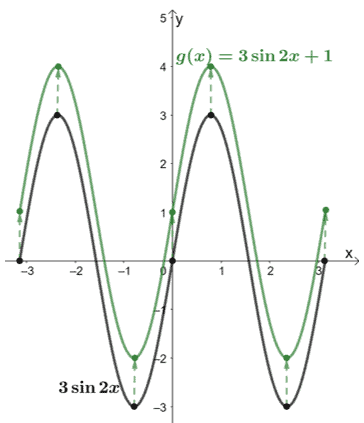
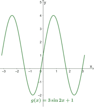
After performing the horizontal compression and vertical stretch on f(x), let’s move the graph one unit upward.
Hence, we have the g(x) graph just by transforming its parent function, y = sin x.
Practice Questions
Images/mathematical drawings are created with GeoGebra.