Vertical Compression – Properties, Graph, & Examples
 Is it possible for us to transform a function by shrinking it down? Yes! One of the most helpful transformation techniques you’ll encounter is vertical compression.
Vertical compression helps us shrink down functions vertically. But by how much? It depends on the scale factor.
Before we start diving deeper into this topic, let’s make sure that we’re equipped with the right techniques and knowledge reviewing the following topics:
- Understanding the common parent functions we might encounter.
- Refresh your knowledge of vertical and horizontal transformations.
- Learn how to apply vertical and horizontal stretches as well.
This article will show how to identify vertical compressions given two or more functions’ expressions and graphs. We’ll also apply our knowledge on vertical compressions by graphing different types of functions.
What is a vertical compression?
Vertical compressions occur when a function is multiplied by a rational scale factor. The base of the function’s graph remains the same when a graph is compressed vertically. Only the output values will be affected.
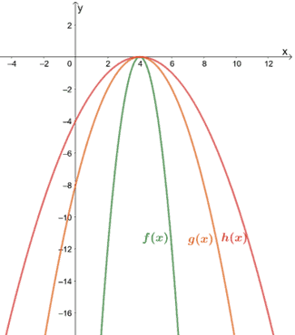
Why don’t we observe what happens when f(x) is vertically compressed by a scale factor of 1/2 and 1/4?
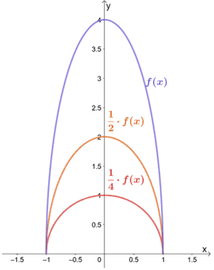
As we may have expected, when f(x) is compressed vertically by a factor of 1/2 and 1/4, the graph is also compressed by the same scale factor.
In general, when a function is compressed vertically by a (where 0 < a < 1), the graph shrinks by the same scale factor. Let’s apply the concept to compress f(x) = 6|x| + 8 by a scale factor of 1/2.
To compress f(x), we’ll multiply the output value by 1/2.
1/2 ∙ f(x) = 1/2 (6|x| + 8)
= 3|x| + 4
Now, what happens with the coordinates of a function that’s compressed by a scale factor of a, where 0 < a < 1? If the base function passes through the point (m, n), the vertically compressed function will pass through the point (m, an).
How to vertically compress a function? We’ve now understood how vertical compression affects a base function. Now, how do we apply this technique when we are given a function’s graph?
Here are some of the important concepts to remember when we transform graphs and compress them vertically:
- Only the values of the y-coordinates will change by a scale factor of a (check if a is a fraction).
- Use critical points and some ordered pairs to guide you in compressing a graph.
- Retain the x-intercept/s of the graph, but the y-intercept will also decrease by a scale factor of a.
Why don’t we try compressing y = 4(x- 4) by a scale factor of 1/4?
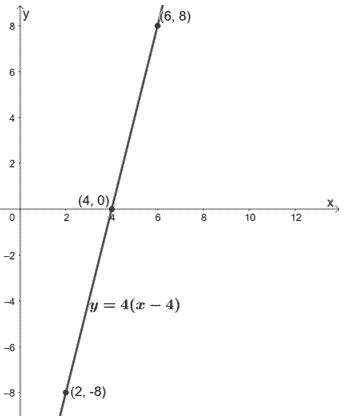
As we have mentioned, it’s important to check for reference points and make sure they can get scaled with the right factor. If we want to compress y = 4(x- 4) by a scale factor of 1/4, we’ll have the following points:
- (2, -8) → (2, -2)
- (6, 8) → (6, 2)
- The x-intercept (4, 0) will remain the same.
Once we have some of the new compressed graph points, let’s graph the transformed function.
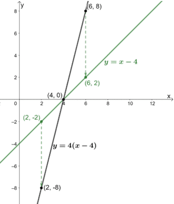
From this, we can see that when y = 4(x – 4) is compressed by a scale factor of 1/4, the new function is equal to y = x – 4.
We can apply the same process when vertically compressing other functions. But first, why don’t we recap what we have learned so far before we try other functions and graphs?
Summary of vertical compression definition and properties
Here are some important reminders when vertically compressing a given function’s graph or expression:
- When 0 < a < 1, af(x) will return a vertically compressed graph with a scale factor of a.
- Apply this concept with the function’s coordinate, so (m, n) becomes (m, an).
- The value and position of the x-intercept/s are the same.
- When f(x) is compressed vertically, its domain will remain constant, but its range may change.
We’re now ready to try out more examples and apply our new knowledge on vertical compressions. Don’t forget to review your notes!
Example 1
The table of values for f(x) is shown below. If h(x) = 1/2 ∙ f(x), construct a table of values for the function h(x).
| x | -3 | -2 | -1 | 0 | 1 | 2 | 3 |
| f(x) | 20 | 10 | 4 | 2 | 4 | 10 | 20 |
Solution
Let’s start with one of the ordered pairs from f(x): (1, 2). Since we want to compress f(x) vertically by 1/2, we’ll multiply the y-coordinate by the same factor.
(1, 2) → (1, 1)
Use the same reasoning to complete the rest of the table of values for h(x).
| x | -3 | -2 | -1 | 0 | 1 | 2 | 3 |
| f(x) | 10 | 5 | 2 | 1 | 2 | 5 | 10 |
Example 2
Use the graph shown below to express the relationships between the three.
a. What is the relationship shared between g(x) and f(x)?
b. What is the relationship shared between g(x) and h(x)?
c. What is the relationship shared between f(x) and h(x)?
Solution
We can check for some reference points to observe the vertical compressions done on each of the graphs.
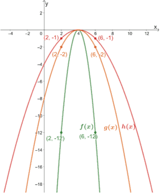
a. Let’s first observe f(x) and g(x). We can see that g(x) is taller than f(x), so a vertical compression is applied on g(x). Checking their points, we have:
(2, -2) → (2, -12) and (6, -2) → (6, -12)
From the two pairs, we can see that f(x) is when g(x) is vertically compressed by a scale factor of 1/6.
b. Let’s apply the same process for g(x) and h(x). From inspection, we know that g(x) is the result of h(x) being vertically compressed. But by what factor? We’ll see.
(2, -1) → (2, -2) and (6, -1) → (6, -2)
Hence, h(x) is when g(x) is vertically compressed by a scale factor of 1/2.
c. Observe the two pairs of points to find the scale factor shared between f(x) and h(x).
(2, -1) → (2, -12) and (6, -1) → (6, -12)
From this, we can see that h(x) is the result when f(x) is vertically compressed by a scale factor of 1/12.
Example 3
Graph the parent function of g(x) = 1/4 ∙ √x. On the same graph, plot g(x) using vertical compressions.
Solution
We’ve already learned that the parent function of square root functions is y = √x. Let’s go ahead and graph y = √x first.
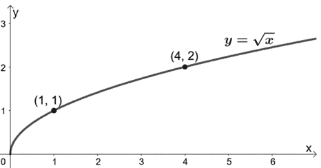
We’ve added some ordered pairs as guides once we graph g(x). Since we want to compress it vertically, we’ll divide the y-coordinates of the parent function by 4.
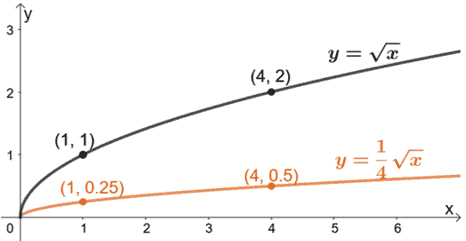
Hence, we have g(x) represented by the orange graph.
Example 4
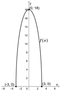
Graph f(x) = 6 √(9 – x2) by finding its intercepts. On the same coordinate system, graph g(x) and h(x) given the following conditions:
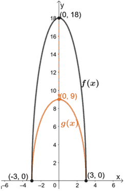
- The function g(x) is the result of f(x) being vertically compressed by a factor of 1/2.
- The function h(x) is the result of g(x) being vertically compressed by a factor of 1/3.
Solution
As suggested, let’s go ahead and find the x and y-intercepts of f(x).
| x | -3 | 0 | 3 |
| f(x) | 0 | 18 | 0 |
Let’s go ahead and plot these intercepts as well as the graph of f(x).
Now that we have f(x)’s graph let’s use the fact that g(x) is the result of vertically compressing f(x) by 1/2. This makes the y-intercept of g(x) as (0, 9).
Let’s now continue graphing h(x) by scaling g(x) vertically by 1/3. This results in h(x) having a y-intercept by (0, 3).
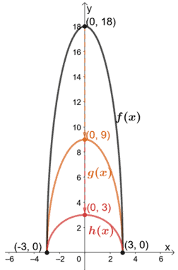
We now have the three functions f(x), g(x), and h(x) on one coordinate system. This problem also confirms that the base of the function’s graph and x-intercepts will remain the same.
Example 5
Describe the transformations done for each pair of functions.
a. g(x) = 3x2 → h(x) = x2/15
b. g(x) = 12x + 4 → h(x) = 3x + 1
c. g(x) = 8|x – 2| – 4 → h(x) = |x -2| – 3
Solution
a. For us to transform g(x) to h(x), we’ll need to divide g(x) by 45: h(x) = g(x) /45. This means that, for us to reach h(x), we need to vertically compress g(x) by a scale factor of 1/45.
b. Dividing g(x) by 4 will result to (12x + 4)/4 = 3x + 1, so h(x) is the result of g(x) being vertically compressed by a scale factor of 1/4.
c. For us to have the expression in h(x), let’s divide g(x) by 4 and subtract 2 from the result. We have h(x) = 1/4 ∙ g(x) – 1, so h(x) is the result of two transformations on f(x): vertically compress it by 1/4 and translate the resulting function 1 unit downward.
Practice Questions
Images/mathematical drawings are created with GeoGebra.