JUMP TO TOPIC
Parametric Curves – Definition, Graphs, and Examples
 Learning about parametric curves will give us one more with special attributes (time to be specific). There are instances when modeling quantities using parametric curves is more helpful than graphing them in the coordinate systems that we know – rectangular and polar coordinate systems. This is why it’s important that we learn how to graph and interpret parametric curves.
Parametric curves allow us to graph relationships between two or more quantities and at the same time represent each quantity’s directions or orientations.
In this article, we’ll take a look back at what we know of parametric equations so far. We’ll also establish the fundamentals needed to parametrize and graph parametric curves. By the end of this discussion, you’ll have the essential tool kits to graph common plane curves to their parametric form. We’ll also show you how some conics in a planar curve can be defined by simpler parametric curves.
What is a parametric curve?
The parametric curve is defined by its corresponding parametric equations: $x = f(t)$ and $y = g(t)$ within a given interval. Parametric curves highlight the orientation of each set of quantities with respect to time.
In the rectangular coordinate system, we are limited to defining functions, $y = f(x)$, that pass the vertical line test. If you’ve noticed, we’ve been working with graphs such as the circle or ellipse that clearly do not pass the vertical line test.
Not being able to define circles and other intersecting curves (like the one shown above) as one function becomes problematic when we deal with its rates of change later. This is why it’s important that we establish a new approach to define such curves.
\begin{aligned}x &= f(t)\\ y &= g(t)\end{aligned}
We begin by defining our variables, $x$ and $y$, through a new parameter – $t$. Hence, the two equations shown above are what we call parametric equations. The points, $(x, y) = (x(t), y(t))$, are the points that make up the graph of a parametric curve. Now how does $t$ affect our curve? The new parameter, $\boldsymbol{t}$, determines the curve’s direction.
| Parametric Curves and Its Endpoints |
\begin{aligned}x &= f(t)\\y &= g(t)\end{aligned} If we have the two plane curves redefined as parametric curves within the interval, $[a, b]$, the parametric curve will have initial points and terminal points at $(x(a),y(a))$ and $(x(b), y(b))$, respectively. |
To motivate you to master this topic, even more, let us write down three major advantages of using parametric curves:
- It is a great model that highlights the direction and orientation of $(x, y)$ based on $t$. This means that we now have a way to model physical representations of quantities that depend on time.
- It is much easier to adjust the parametric curve if we want to change the value of $t$ or we want to switch the orientations.
- There are instances when curves such as implicit curves can only be modeled by parametric equations (ie modeling both the volume of a container and its spillage simultaneously with respect to time).
Now that we have established the importance of parametric curves as well as their key components, let’s refresh our understanding of parametrizing equations and their graphs.
How to parametrize a curve?
When given a plane curve, we can parametric it to a parametric curve by redefining $x$ and $y$ as a set of parametric equations defined by $t$. There are infinitely many ways to parametrize a given curve – what matters is that their definition as a plane curve remains the same. The simplest way to parametrize a curve is by setting $x = t$.
PARAMETRIZING A PLANE CURVE The most straightforward option when parametrizing a plane curve defined by $y = f(x)$ is to use the following parametric equations: \begin{aligned}x &= t\\y&= f(t)\end{aligned} Keep in mind that $t$ has to be within the domains of $f(x)$. |
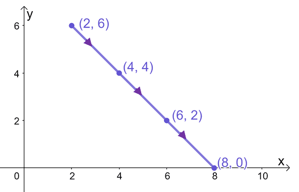
This strategy works when we want to parametrize a line. We simply use $x = t$ and $y = mt + b$. This allows us to observe the behavior of the curve as $t$ increases. However, there are instances when it’s best to strategize when choosing the right parametric equations. Let us show you the standard way we redefined equations of circles using parametric equations:
PARAMETRIZING CIRCLES We can parametrize a circle centered at the origin using the following parametric equations: \begin{aligned} x &= r\cos t \\ y &= r \sin t \end{aligned} Circles centered at $\boldsymbol{(h, k)}$ using the following parametric equations: \begin{aligned} x &= h + r\cos t \\ y &= k + r \sin t\end{aligned} For both cases, keep in mind that $0 \leq t \leq 2\pi$. |
These are two of the most common curves we usually parametrize and it’s best if you master their general parametric forms to save you time later on. Of course, the idea remains the same for the rest of the plane curves – as long as our defined parametric curves still represent the same plane curves and $t$ is within the set domain.
We can also reverse the process of parametrization by eliminating the parameters. We simply apply our algebraic technique to eliminate $\boldsymbol{t}$ in the equations, $x = f(t)$ and $y = g(t)$.
- Isolate $t$ from one of the parametric equations.
- Use the resulting expression (either in terms of $x$ or $y$) to eliminate the parameter in the remaining parametric equation.
Let’s try eliminating the parameter from the curve of $x = t^2 – 4$ and $y = 4t$ where $-4 \leq t\leq 4$. It’s easier to isolate $t$ in $y= 2t – 4$. Hence, we have $t = \dfrac{y}{4}$. Substitute this expression into $x = t^2– 4$, we have:
\begin{aligned} x &= t^2 – 4\\&= \left(\dfrac{y}{4}\right)^2 -4\\&= \dfrac{y^2}{16} – 4\end{aligned}
We can rewrite this equation as $y^2 = 4(x +16)$ – a parabola with vertex at $(-4, 0)$. Eliminating parameters is helpful when we want to understand or predict a parametric curve’s shape using our knowledge of plane curves.
How to graph a parametric curve?
Now that we know how to parametrize curves, it’s time that we establish the steps we need to graph parametric curves. Below are helpful guidelines for you to remember when y graphing parametric curves given their parametric equations:
- Assign some key values of $t$ within the given interval.
- Use the parametric equations, $x = f(t)$ and $y= g(t)$, to find the corresponding ordered pairs, $(x, y)$.
- Plot the ordered pairs in order – start with the ordered pair returned by the lowest value of $t$ up to the highest value of $t$.
We’ve actually shown examples of the graphing parametric curves of a linear function and circles in the linked articles. Take a quick look at them if you want examples of graphing these two most common parametric curves.
For now, let’s go back to our parametric equations – $x = t^2 – 4$ and $y = 4t$, where $t$ is within $[-4, 4]$. First, we assign key values for $t$. Ideally, these are values that are easy to work with given our parametric equations. Hence, we choose $t = \{-4, -2, 0, 2, 4\}$. Substitute each value of $t$ into our two parametric equations. We’ve summarized the calculations done in one table – ideally, start from the lowest value of $t$ to the highest one.
| \begin{aligned}\boldsymbol{t}\end{aligned} | \begin{aligned}\boldsymbol{x = t^2 – 4}\end{aligned} | \begin{aligned}\boldsymbol{y = 4t}\end{aligned} | \begin{aligned}\boldsymbol{(, y)}\end{aligned} |
| \begin{aligned}-4\end{aligned} | \begin{aligned}x= (-4)^2 – 4 = 12\end{aligned} | \begin{aligned}y = 4(-4) = -16\end{aligned} | \begin{aligned} (12, -16)\end{aligned} |
| \begin{aligned}-2\end{aligned} | \begin{aligned}x= (-2)^2 – 4 = 0\end{aligned} | \begin{aligned}y = 4(-2) = -8\end{aligned} | \begin{aligned} (0, -8)\end{aligned} |
| \begin{aligned}0\end{aligned} | \begin{aligned}x = 0^2 – 4 = -4\end{aligned} | \begin{aligned}y = 4(0) = 0\end{aligned} | \begin{aligned} (-4, 0)\end{aligned} |
| \begin{aligned}2\end{aligned} | \begin{aligned}x = 2^2 – 4 = 0\end{aligned} | \begin{aligned}y = 4(2) = 8\end{aligned} | \begin{aligned} (0, 8)\end{aligned} |
| \begin{aligned}4\end{aligned} | \begin{aligned}x = 4^2 – 4 = -12\end{aligned} | \begin{aligned}y = 4(4) = 16\end{aligned} | \begin{aligned} (-12, 16)\end{aligned} |
Plot these points on the $xy$-plane then connect them with a smooth curve. Include arrows along the curve to highlight the direction of the curve from $t = -4$ to $t= 4$.
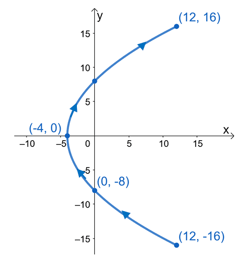
Make sure to plot the ordered pairs in order starting from $t = -4, (12, -16)$ to $t = 4, (12, 16)$. This will help you remember the direction of the parametric curve and make it easier for you to label the arrows and highlight the curve’s direction.
As we have predicted, the curve of the equation is a parabola centered at $(-4, 0)$. This highlights the importance of knowing how to eliminate parameters to predict the shape of the parametric curve.
How to find the derivative of parametric curves?
We can find the parametric curves’ derivative by applying the chain rule and other derivative rules. Now that we have explored the basic concepts of parametric curves, let’s take a deeper understanding by seeing parametric curves in the context of calculus.
We begin by assuming that $\dfrac{dx}{dt} = f^{\prime}(t) $ and $\dfrac{dy}{dt} = g^{\prime}(t)$ exist and that $f^{\prime}(t) \neq 0$. This means that we can express $\dfrac{d}{dx} g(x) = \dfrac{dy}{dx}$ as shown below.
\begin{aligned}\dfrac{dy}{dx} &= \dfrac{dy/ dt}{dx/ dt}\\&= \dfrac{g^{\prime}(t) }{f^{\prime}(t)}\end{aligned}
DERIVATIVE OF PARAMETRIC CURVE \begin{aligned}x & = f(t)\\ y&= g(t) \end{aligned} We can find the derivative of the parametric curve represented by the parametric equations shown above by dividing the derivative of $g(t)$ by the derivative of $f(t)$- both with respect to $t$. \begin{aligned}\dfrac{dy}{dx} &= \dfrac{g^{\prime}(t)}{f^{\prime}(t)}\end{aligned} |
When an equation is in its parametric form, we can find the coordinates of its critical points by finding the values of $\boldsymbol{t}$ where $\boldsymbol{\dfrac{dy}{dx}}$ is equal to zero or are undefined. We can use the derivative of parametric curves as their critical points to graph parametric curves faster.
Why don’t we try to find the derivative of the parametric curve , $x = t^2 – 4$ and $y = 4t$? Take their individual derivatives with respect to $t$ then use thhe formula, $\dfrac{dy}{dx} = \dfrac{g^{\prime}(t)}{f^{\prime}(t)}$.
| \begin{aligned} f^{\prime}(t) &= \dfrac{d}{dt} (t^2 – 4) \\ &= 2t^{2 – 1} – 0\\&= 2t \\g^{\prime}(t) &= \dfrac{d}{dt} (4t) \\&= 4(1) \\&= 4 \end{aligned} | \begin{aligned} \dfrac{dy}{dx} &= \dfrac{g^{\prime}(t)}{f^{\prime}(t)} \\&= \dfrac{4}{2t}\\ &= \dfrac{2}{t}\end{aligned} |
From this, we can see that $\dfrac{dy}{dx}$ is undefined when $t = 0$, so the critical point of the function is located at $t = 0$. Using the table of values from the previous section, we can see that when $t = 0$, $(x, y) = (-4, 0)$ which is the turning point of the parametric curve.
When we know the critical points of a parametric curve, we can save our time point-plotting parametric curves. We can instead use the endpoints and the critical points to graph the parametric curve.
Don’t worry we’ve prepared more problems for you to work on and test your knowledge on parametric curves. Go through the article once more and when you’re ready, head over to the next section!
Example 1
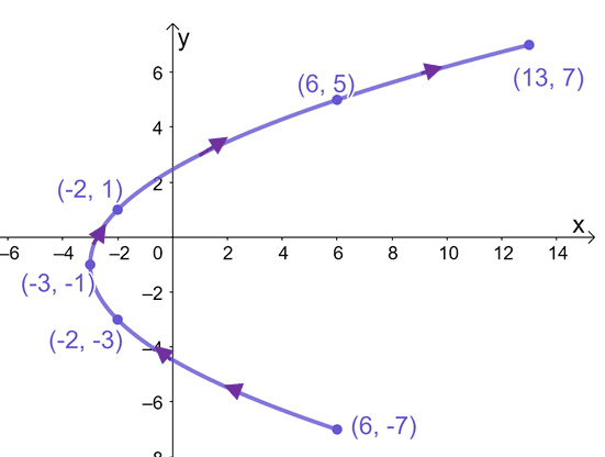
Graph the curve defined by the parametric equations $x = 2\sqrt{t}$ and $y = t- 2$, where $t \geq 0$. Include arrows showing the orientation of the resulting parametric curve.
Solution
We begin by assigning integral values of $t$ that are greater than or equal to $0$. Evaluate each of the values at $x = 2\sqrt{t}$ and $y = t- 2$ to find some ordered pairs that will help us in plotting the parametric curve. Here’s the summary of our calculations when $t = \{0, 1, 4, 9, 16\}$.
| \begin{aligned}\boldsymbol{t}\end{aligned} | \begin{aligned}\boldsymbol{x = 2\sqrt{t}}\end{aligned} | \begin{aligned}\boldsymbol{y = t- 2}\end{aligned} | \begin{aligned}\boldsymbol{(, y)}\end{aligned} |
| \begin{aligned} 0\end{aligned} | \begin{aligned}x = 2\sqrt{0} = 0\end{aligned} | \begin{aligned}y = 0 -2= -2\end{aligned} | \begin{aligned} (0, -2)\end{aligned} |
| \begin{aligned}1\end{aligned} | \begin{aligned}x = 2\sqrt{1} = 2\end{aligned} | \begin{aligned}y = 1 -2= -1\end{aligned} | \begin{aligned} (2, -1)\end{aligned} |
| \begin{aligned}4\end{aligned} | \begin{aligned}x = 2\sqrt{4} = 4\end{aligned} | \begin{aligned}y = 4 -2= 2\end{aligned} | \begin{aligned} (4, 2)\end{aligned} |
| \begin{aligned}9\end{aligned} | \begin{aligned}x = 2\sqrt{9} = 6\end{aligned} | \begin{aligned}y = 9 -2= 7\end{aligned} | \begin{aligned} (6, 7)\end{aligned} |
| \begin{aligned}16\end{aligned} | \begin{aligned}x = 2\sqrt{16} = 8\end{aligned} | \begin{aligned}y = 16 -2= 14\end{aligned} | \begin{aligned} (8, 14)\end{aligned} |
Now, plot the five ordered pairs on an $xy$-plane then connect them with a smooth curve.
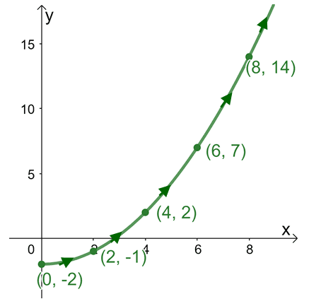
This represents the parametric curve, $x = 2\sqrt{t}$ and $y = t- 2$, and don’t forget to include the arrows to highlight the curve’s orientation when.
Example 2
Eliminate the parameter for the parametric equations, $x= \sec t$ and $y = \tan t$. Use the resulting rectangular equation to graph the plane curve. Include arrows showing the orientation of the resulting parametric curve.
Solution
It’ll be easier for us to eliminate the parameter if we square both parametric equations. By doing so, we can express $\sec^2 t$ in terms of $\tan^2 t$ and vice-versa.
| \begin{aligned}(x)^2 &= (\sec t)^2\\x^2 &= \sec^2 t\end{aligned} | \begin{aligned}(y)^2 &= (\tan t)^2\\y^2 &= \tan^2 t\end{aligned} |
Use the Pythagorean identity, $\tan^2 t + 1 = \sec^2 t$, to rewrite $x$ in terms of $y$.
\begin{aligned}x^2 &= \sec^2 t\\&= \tan^2 t + 1\\x^2 &= y^2\end{aligned}
We’ve now eliminated the parameter, $t$, and by isolating all terms on the left-hand side of the equation, we have $x^2 – y^2 = 0$. This is in fact a hyperbola centered at $(0, 0)$ and with vertices at $(-1, 0)$ and $(1, 0)$.
To know the direction of the plane curve, let’s evaluate $t$ at different values to find some ordered pairs from $t = 0$ to $t = 2\pi$.
| \begin{aligned}\boldsymbol{t}\end{aligned} | \begin{aligned}\boldsymbol{x = \sec t}\end{aligned} | \begin{aligned}\boldsymbol{y = t- 2}\end{aligned} | \begin{aligned}\boldsymbol{(, y)}\end{aligned} |
| \begin{aligned} 0\end{aligned} | \begin{aligned}x = \sec 0 = 1\end{aligned} | \begin{aligned}y = \tan 0= 0\end{aligned} | \begin{aligned} (1, 0)\end{aligned} |
| \begin{aligned}\dfrac{\pi}{3}\end{aligned} | \begin{aligned}x = \sec \dfrac{\pi}{3} =2\end{aligned} | \begin{aligned}y = \tan \dfrac{\pi}{3}= \sqrt{3}\end{aligned} | \begin{aligned} (2, 1.73)\end{aligned} |
| \begin{aligned}\dfrac{2\pi}{3}\end{aligned} | \begin{aligned}x = \sec \dfrac{2\pi}{3} =-2\end{aligned} | \begin{aligned}y = \tan \dfrac{2\pi}{3}= -\sqrt{3}\end{aligned} | \begin{aligned} (-2, -1.73)\end{aligned} |
| \begin{aligned} \pi\end{aligned} | \begin{aligned}x = \sec \pi = -1\end{aligned} | \begin{aligned}y = \tan \pi= 0\end{aligned} | \begin{aligned} (-1, 0)\end{aligned} |
| \begin{aligned}\dfrac{4\pi}{3}\end{aligned} | \begin{aligned}x = \sec \dfrac{4\pi}{3} =-2\end{aligned} | \begin{aligned}y = \tan \dfrac{4\pi}{3}= \sqrt{3}\end{aligned} | \begin{aligned} (-2, 1.73)\end{aligned} |
| \begin{aligned}\dfrac{5\pi}{3}\end{aligned} | \begin{aligned}x = \sec \dfrac{5\pi}{3} =2\end{aligned} | \begin{aligned}y = \tan \dfrac{5\pi}{3}= -\sqrt{3}\end{aligned} | \begin{aligned} (2, -1.73)\end{aligned} |
Plot these ordered pairs and connect them with a smooth curve. Of course, this example is tricky since the points are scattered throughout the four quadrants. This is why eliminating parameters can be helpful – we’ll use the fact that the resulting plane curve is a hyperbola to graph the curve correctly.
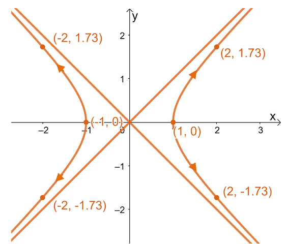
This is a great example of a conic section’s parametrization. As you can see, finding ordered pairs using the parametric form is easier than directly finding ordered pairs using the rectangular form. This becomes more apparent when working with more complex conic sections.
Example 3
Write down two different sets of parametric equations to parametrize the equation, $y = 3x + 5$.
Solution
Before we begin, remember that rectangular equations can be represented by multiple sets of parametric equations. This means that we may show different sets of parametric equations than what you might write down. What matters is that your set of parametric equations return $y = 3x + 5$ when we eliminate the parameter, $t$.
For our two sets of parametric equations, we’ll let 1)$x$ be equal to $t$ and 2)$x$ be equal to $ t +1$. We’ll substitute each of this equation into the rectangular equation.
| \begin{aligned}\boldsymbol{x = t }\end{aligned} | \begin{aligned}\boldsymbol{x = t + 1 }\end{aligned} |
| \begin{aligned}y &= 3(t) + 5\\&= 3t + 5 \end{aligned} | \begin{aligned}y &= 3(t +1) + 5\\&= 3t + 8\end{aligned} |
This means that the equation, $y = 3x + 5$, can be expressed as the following sets of parametric equations: $x = t, y = 3t + 5$ and $x = t + 1, y = 3t + 8$.
Example 4
Find the derivative of the plane curve defined by the equations, $x = 2t + 1$ and $y = t^3 – 27t$ where $t$ is within $[-5, 10]$, then use the result to find the plane curve’s critical points.
Solution
Take the derivative of each parametric equation with respect to $t$.
| \begin{aligned}\boldsymbol{x = 2t + 1 }\end{aligned} | \begin{aligned}\boldsymbol{y = t^3 -27t}\end{aligned} |
| \begin{aligned}\dfrac{dx}{dt} &= 2(1) \\&= 2\end{aligned} | \begin{aligned}\dfrac{dy}{dt} &= 3t^2 – 27(1) \\&= 3t^2 – 27\end{aligned} |
Use the formula, $\dfrac{dy}{dx} = \dfrac{ dy/dt}{ dx/dt}$, to find the derivative of the plane curve. Hence, we have $\dfrac{dy}{dx} = \dfrac{3t^2 – 27}{2}$.
The derivative is zero when $t = \pm 3$, so evaluate the parametric equations at $t= -3$ and $t=3$ to find the critical points.
| \begin{aligned}\boldsymbol{t=-3 }\end{aligned} | \begin{aligned}\boldsymbol{t = 3}\end{aligned} |
| \begin{aligned}(x, y) &= (-5, 6) \end{aligned} | \begin{aligned}(x, y) &= (7, 18) \end{aligned} |
This means that the plane curve has critical points at $(-5, 6)$ and $(7, 18)$.
Practice Questions
1. Graph the curve defined by the following parametric equations using point-plotting. Include arrows showing the orientation of the resulting parametric curve.
a. $x = t + 4$, $y = 4- 2t$; $-2 \leq t \leq 4$
b. $x = t^2-3$, $y = 2t -1$; $-3 \leq t \leq 4$
c. $x =\sqrt{t}$, $y = t +4$; $ t \geq 0$
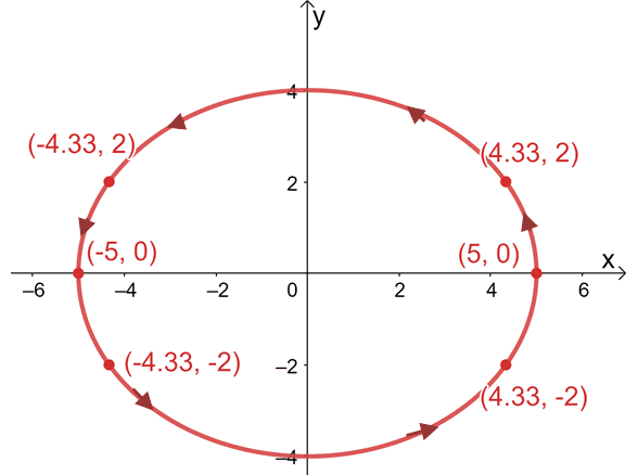
2. Eliminate the parameter for the parametric equations, $x= 5\cos t$ and $y = 4\sin t$. Use the resulting rectangular equation to graph the plane curve. Include arrows showing the orientation of the resulting parametric curve.
3. Write down two different sets of parametric equations to parametrize the following equations.
a. $y = 2x – 9$
b. $y = x^2+1$
c. $y = x^2–5$
Answer Key
1.
a.
b.
c.
2.
$\dfrac{x^2}{25} + \dfrac{y^2}{4} = 1$
3. These are just sample answers. It’s okay if you have different sets of parametric equations.
a. $y = 2x – 9$ : $\{x = t, y= 2t – 9\}$ and $\{x = 4t, y = 8t -9\}$
b. $y = x^2 + 1$: $\{x = t,y= t^2 + 1\}$ and $\{x=-2t, y = 4t^2 +1\}$
c. $y = x^2 – 5$: $\{x = t, y= t^2 – 5\}$ and $\{x=3t, y = 9t^2 -5\}$
Images/mathematical drawings are created with GeoGebra.