JUMP TO TOPIC
Polynomial Functions – Properties, Graphs, and Examples
 If you’ve been working with functions, you would already have been dealing with polynomial functions as well. These are also among the most used functions in real-world models and are considered one of Algebra’s “building blocks.” With its extensive application, we should study and understand polynomial functions, starting with their definition.
Polynomial functions are functions that term or terms that may contain different components, including variables, constant, and exponents.
Try to think of different combinations, and you’ll realize that polynomial functions cover a wide number of functions.
This is why this article will be thorough in discussing the different aspects of polynomial functions. We’ll discuss the following:
- Identifying common polynomial functions.
- Predicting the end behavior and graphing polynomial functions.
- Manipulating and finding polynomial functions.
- Modeling and interpreting polynomial functions.
Make sure to take notes as learning about polynomials and their graphs can help us understand different functions and real-world mathematical models.
What is a polynomial function?
Let’s break down the word polynomial into two: poly and nomial. The first means many, and the second means term, so when combined, polynomials are expressions with many terms.
Here’s the general form of polynomials:
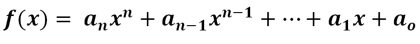
Note that an, an-1, … ao can be any complex number (except for an since it can’t be equal to zero).
In the next section, we’ll learn how to break down each term and further understand how we can modify and manipulate the general form of polynomial functions.
Polynomial function definition and examples
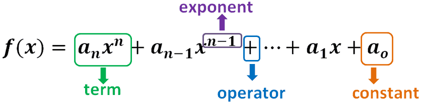
From the general form of the polynomial function, we can see that polynomials are expressions that are made up of constants, variables, operators, and nonnegative exponents.
Why don’t we break down the general formal components and identify common elements that we can find in a polynomial function?
Note that an, an-1, … ao can be any complex number (except for an since it can’t be equal to zero).
In the next section, we’ll learn how to break down each term and further understand how we can modify and manipulate the general form of polynomial functions.
Polynomial function definition and examples
From the general form of the polynomial function, we can see that polynomials are expressions that are made up of constants, variables, operators, and nonnegative exponents.
Why don’t we break down the general formal components and identify common elements that we can find in a polynomial function?
In general, the terms of polynomials contain nonzero coefficients and variables of varying degrees. The leading term of f(x) is anxn, where n is the polynomial’s highest exponent.
Polynomials also contain terms with different exponents (for polynomials, these can never be negative). More often than not, polynomials also contain constants. These are the whole numbers we normally see at the end of a polynomial expression.
Let’s go ahead and list down some examples of polynomials and identify these different components.
| Examples | Variables | Exponents | Constants | Terms |
| 4mn2 – 2mn + n3 – 12 | m and n | 2 in 4mn2 3 in n3 | -12 | 4mn2, 2mn, ,n3, and 12 |
| x2 – 6x + 9 | x | 2 in x2 1 in 6x | 9 | x2, 6x, and 9 |
| xy3 – x2y2 + 16 | x and y | 3 in xy3 | 16 | xy3, x2y2, and 16 |
You can list more if you like and practice identifying their different components. For now, let’s go ahead and understand the properties we might encounter from polynomial functions.
What are the degrees and leading coefficients of polynomials?
When dealing with polynomials, you’ll encounter the term degree. Degrees will help us predict the behavior of polynomials and can also help us group polynomials better.
Degrees return the highest exponent found in a given variable from the polynomial. For example, if we have y = -4x3 + 6x2 + 8x – 9, the highest exponent found is 3 from -4x3. This means that the degree of this polynomial is 3.
What if our polynomial has terms with two or more variables? Then, its degree will depend on the highest sum of the exponents from each term.
Why don’t we observe 6x2y2 + 3xy3 – 5x2y4 + 6? Let’s find the sum of the exponents of each term:
- The sum of the exponents from 6x2y2 is 2 + 2 =
- Similarly, the sum of the exponents from 3xy3 is also 1 + 3 = 4.
- Lastly, the sum of the exponents from 5x2y4 is 2 + 4 = 6.
From this, we can see that the highest sum is 6, so the given polynomial has a degree of 6. We call the term containing the highest degree as the polynomial’s leading coefficient, so for this case, it’s 5x2y4.
Getting the hang out it? Why don’t we try out finding the degrees and the leading coefficients of these polynomials shown below?
| Polynomial | Degree | Leading Coefficient |
| 5x4 + 6x3 – 3x2 + 1 | 4 | 5x4 |
| 4mn3 – 3m2n4 + mn6 | 7 | mn6 |
| 24a2b3 – 12a4b2 + 120a8 | 8 | 120a8 |
Now that we’ve learned about polynomials and their unique components, it’s time that we learn how we can classify common polynomials based on their degrees and number of terms.
What are the common types of polynomial functions?
With the extensive number of polynomials and polynomial functions we might encounter, we should learn how we can classify the most common types of polynomial functions.
Let’s start with classifying polynomial functions based on their number of terms.
The three most common polynomials you might encounter are monomials, binomials, and trinomials.
- Monomials are polynomials that only contain one term.
- Examples: -5x2, 23a, and 6y3
- Binomials are polynomials that contain two terms.
- Examples: a + b, 5x – 2, and 3x + 2y
- Trinomials are polynomials that contain three terms.
- Examples: x2 – 2x + 1, y4 – 6y2 + 9, and mn2 – 2mn + 5mn
Now, let’s classify polynomials based on their degrees.
The four most common polynomials that we’ll be studying in our algebra and precalculus classes are linear, quadratic, cubic, and quartic.
- Linear functions are functions with a degree of 1.
- Examples: 2x + 1, 3y – 1, and a + b
- Quadratic functions are functions with a degree of 2.
- Examples: 4x2 – 1, x2 + 4x + 4, and m2 – 2mn + n2
- Cubic functions are functions with a degree of 3.
- Examples: 2x3, 5y3 – 2y2 + 12, and a3 + ab2 – ab + b3
- Quartic functions are functions with a degree of 4.
- Examples: x4 – y4, x4 – 3x3 + 2x – 4, and a4 – 2x2 + 1
How to graph a polynomial function?
We may have graphed simpler polynomial functions such as linear, quadratic, and power functions in the past, so it’s best to review your notes to recall the different types of graphs we’ve learned in the past.
But what if we’re given a polynomial function with a degree greater than two or a more complex expression? Here are some helpful tips to remember when graphing polynomial functions:
- Graph the x and y-intercepts whenever possible.
- Determine the end behavior of the function.
- Find the number of turning points that a function may have.
- Apply transformations of graphs whenever possible.
Don’t worry. We’ll get into these properties slowly, and understanding each of these components can help us graph polynomial functions.
Finding the Intercepts
The y-intercept can be determined right away by setting x to 0.
Some polynomial functions may be in a factored form already, so equate each factor to 0 right away to find the x-intercepts? But, what if we’re given a complex polynomial function? No worries, we’ve written a special article on how to solve polynomial equations here.
Make sure to plot these intercepts right away as a guide when graphing the polynomial function’s curve.
Behavior at the Zeros
Once we have the x-intercepts or the zeros of the function, we can predict how the curve behaves at these zeros depending on its multiplicity.
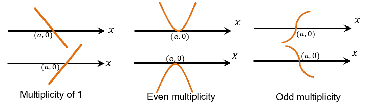
Let’s go ahead and go through each of the three cases:
- If the zero has a multiplicity of 1, the graph passes through the x-axis once.
- If the zero has an even multiplicity, the curve bounces or turns at the x-intercept.
- Suppose the zero has an odd multiplicity, the curve bounce cross and turns at the x-axis. This results in curves looking like curves, as shown above.
End Behaviors and Turning Points
Let’s start with turning points. We can predict the maximum number of turning points by their degree.
- If the function has n degrees, the maximum number of points present in the graph is n – 1.
- We’re also expecting the graph to contain turning points in between two x-intercepts.
As for end behaviors, these will depend on the leading term of the polynomial. If the polynomial function has a leading term of axn, the end behavior will depend on whether n is odd or even and if a is positive or odd.
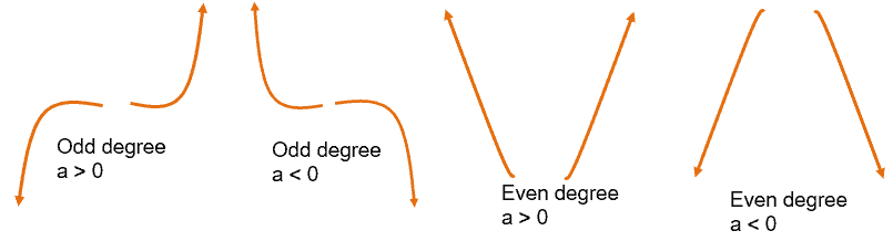
The guide above can help us know what to expect at the ends of the curve.
- When the degree (n) is odd, both ends will either increase or decrease depending on whether the coefficient (or a) is positive or negative.
- When n or the degree is even, one end is increasing while the other end is decreasing. The order will depend on the coefficient (a)’s sign.
Aside from these properties, make sure to review what we know about transformations and power functions. Use these whenever possible to also save time when graphing functions.
How to solve polynomial functions?
Since polynomial functions contain an extensive group of functions, we can use a lot of methods when solving polynomial functions.
But the same concept is applied: to solve for the zeroes or solutions of the polynomial function, we equate the expression to 0 and solve for x. Here’s a table to summarize the common methods we can apply when solving polynomial functions.
| Type of Polynomial Function | Method |
| Linear Function | Isolate the variable on one side to solve for its solution. |
| Quadratic Function | Factor the expression and equate each expression to 0. Apply the quadratic formula. |
| Cubic Function | Factor whenever possible and equate each expression to 0. Graphical solution can also be considered. |
| Polynomial Functions (n > 3) | When working with more complex polynomial functions, apply the following concepts to solve for the polynomial function: · Rational zeros theorem · Synthetic division · Factoring |
Don’t worry. We’ve actually written a separate article about solving polynomial equations because it’s important for us to master this concept.
What if we’re given the graph and want to find the polynomial function representing it? We’ll use the same properties we’ve just discussed in the previous section, but we’ll do it in reverse this time.
Let’s first summarize how the different properties would affect the polynomial function’s graph with this guide.
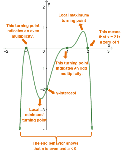
This guide also tells us how from the graph of a polynomial function alone, we can already determine a wide range of information about the polynomial function.
Let’s try finding a function that can represent the graph shown above. Using the multiplicity of the graphs, here are the simplest possible factors of the function, f(x):
f(x) = a(x – – 1)2(x – 1)3(x – 2)
=a(x + 1)2(x – 1)3(x – 2)
We can use these observations and other given information from the problem to find missing polynomial functions and interpret a polynomial model’s behavior.
For the case of f(x), we can use the y-intercept. Substitute x = 0 and f(x) = -2 to solve for a.
-2 = a(0 + 1)2(0 – 1)3(0 – 2)
-2 = a(1)(-1)(-2)
-2 = 2a
a = -6
Hence, we have f(x) = -6(x – 2)(x + 1)2(x – 1)3.
Think you’re ready to test your knowledge on polynomial functions now? Let’s go ahead and answer these problems to check our knowledge.
Example 1
Which of the following functions are considered polynomial functions?
a. f(x) = -2x2 + 3x – 5
b. g(x) = 3√x – 1
c. h(x) = πx2 – π
d. m(x) = 2x + 5/x
e. n(x) = 3 cos x – 1
Solution
Let’s go ahead and observe each function and see if they meet the definition of polynomial functions.
a. Polynomial functions can contain multiple terms as long as each term contains exponents that are whole numbers. Since f(x) satisfies this definition, it is a polynomial function. In fact, it is also a quadratic function.
b. The term 3√x can be expressed as 3x1/2. Its exponent does not contain whole numbers, so g(x) is not a polynomial function.
c. At first glance, we may think that π is not a valid coefficient, but π is a real number, and the exponent of h(x) is a real number, so h(x) is, in fact, a polynomial function.
d. Remember that 5/x can be expressed as 5x-1, so it’s not a whole number. This means that m(x) is not a polynomial function.
e. The term 3 cos x is a trigonometric expression and is not a valid term in polynomial function, so n(x) is not a polynomial function.
Example 2
Determine the degree of the following polynomials.
a. f(x) = 3x3 + 2x2 – 12x – 16
b. g(x) = -5xy2 + 5xy4 – 10x3y5+ 15x8y3
c. h(x) = 12mn2 – 35m5n3 + 40n6 + 24m24
Solution
We can find the degree of a polynomial by finding the term with the highest exponent. The exponent value (or the sum of the exponents) will be the degree of the function.
a. For f(x), we can immediately see that the leading term is 3x3 and the degree of the function is 3.
b. Since g(x) contains terms with multiple variables, make sure to add the exponents found in each variable. We can see that the highest sum of exponents is 11 (from the leading term, 15x8y3. Hence, the degree of g(x) is 11.
c. We apply the same process for the terms of h(x) with two variables. By inspection, we can see that the highest combined exponent is 24 (from 24m24). Hence, the degree of h(x) is 24.
Example 3
Write a function that satisfies the following conditions.
a. It is both a monomial and a cubic function.
b. It has a leading term of 24x3.
c. It is a trinomial with a degree of 5.
Solution
This question can have a lot of possible answers. What matters is that the resulting function satisfies the given conditions.
a. Monomials are polynomials containing one term, while a cubic function is a polynomial function with a degree of 3. So, for a function to satisfy both conditions, our function must only have one term with an exponent of 3.One function that satisfies this is f(x) = -5x3.
This means that any coefficient before x3 will be a valid function.
b. The polynomial function’s leading term is the term that contains the highest exponent (or sum of exponents for multi-variable terms). This means that we want a function with 3 as its highest exponent, so one possible function is g(x) = 24x3 – 24x + 1.
As long as the terms you add have exponents that are less than 3, your answer is correct.
c. Recall that trinomials are functions in three terms. We want a function with a leading term with an exponent of 5 but only contains three terms. We can start with x5 as its leading term and add two more terms. Hence, h(x) = x5 – 3x3 + 1 is one example of this function.
In general, functions that have 5 as their highest exponent and contains three terms would be valid.
Example 4
Illustrate and describe the end behavior of the following polynomial functions.
a. f(x) = 3x5 + 2x3 – 1
b. g(x) = 4 – 2x + x2
c. h(x) = -x6 + 5x2 – 2x + 4
Solution
When predicting the end behavior of a polynomial function, identify the leading term (axn) first. Determine whether its coefficient, a, is positive or negative. Take note of whether the degree (n) of the function is even or odd.
a. The leading term of f(x) is 3x5. We can see that a > 0 and f(x) have an odd degree. From what we’ve learned, we can predict its end behavior to be increasing on both ends.
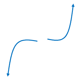
This diagram illustrates the direction of the end curves of f(x).
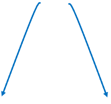
b. The function g(x) has a leading term of x2, so a > 0 and g(x) has an even degree. This means that its curve is decreasing when x < 0 and increasing when x > 0.

This diagram illustrates the direction of the end curves of f(x).
c. The function g(x) has a leading term of x2, so a > 0 and g(x) has an even degree. This means that its curve is decreasing when x < 0 and increasing when x > 0.
This diagram illustrates how the curve of h(x) will behave.
Example 5
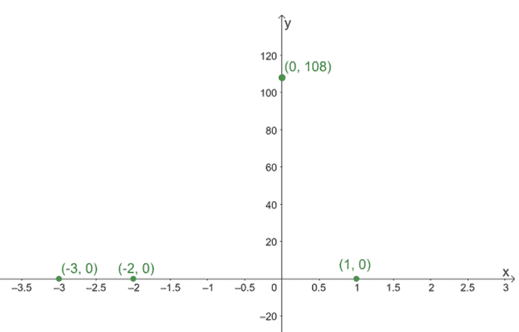
Graph the polynomial function g(x) = -(x – 1)(x + 2)2(x + 3)3. Make sure also to determine the following:
a. The x and y-intercepts of g(x).
b. The behavior of the roots of g(x).
c. The end behavior of g(x).
Solution
Let’s start with g(x)’s intercepts.
- Find the y-intercept of g(x) by setting x = 0. Hence, we have g(0) = -(-1)(2)2(3)3 = 108.
- Find the x-intercept by setting g(x) to 0 and solving for x by equating each factored expression to 0.
x – 1 = 0 x = 1 | x + 2 = 0 x = -2 | x + 3 = 0 x = -3 |
- Hence, g(x) has intercepts at (0, 108), (1,0), (-2, 0), and (-3, 0).
Now, let’s see what we should expect from x-intercepts when the curve passes through the x-axis.
- Since (x – 1) has a multiplicity of 1, the curve will only cross through x = 1 once.
- The factor (x + 2) has a multiplicity of 2; the curve bounces when it passes through x = -2.
- The factor (x + 3) has a multiplicity of 3, the curve bounces and crosses the x-axis at x = -3.
To determine the end behaviour of g(x), let’s find its leading term first: axn = -1(x)(x)2(x)3 = -x6. Since the coefficient is negative and the degree is even, g(x) is increasing when x < 0 and decreasing when x > 0 as demonstrated by the diagram below.
Let’s first plot the intercepts of g(x) as a guide when graphing its curve.
Use the behavior of the graph at the zeros and the end behavior of the graph to plot the curve of g(x).
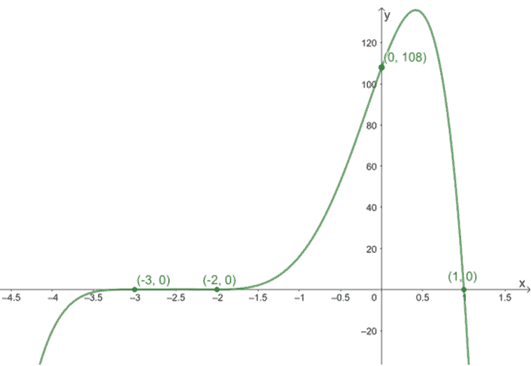
The graph confirms the behavior of the curve as it passes through each of the x-intercepts or zeros.
We can also confirm how the end curves are both going down as we have predicted.
You can also check that there are at most (6 – 1) = 5 turning points in the graph (in fact, we can only see three).
Practice Questions
Images/mathematical drawings are created with GeoGebra.