Differential Equations – Definition, Types, and Solutions

Differential equations open a wide range of applications in mathematics, physics, engineering, and even finance. There are a lot of physical phenomena that are defined through calculus and differential equations. Through differential equations, we can solve equations containing derivatives and initial conditions.

Differential equations combine our knowledge of derivatives, integrals, and algebra to solve equations that contain functions and their derivatives.

Seeing how vital differential equations are in higher mathematics, we must understand the components of differential equations, know the different types of differential equations, and learn how to simplify and solve these types of equations. This article is an introductory article – our goal is to give you an initial impression of differential equations.

What Is a Differential Equation?

To put it simply, a differential equation is an equation that contains one term or more that are ordinary or partial derivatives of the function (or functions) we’re working on. Through differential equations, we can now find the relationship between functions and their derivatives. Here are some examples of differential equations in different orders:

\begin{aligned}\dfrac{dy}{dx} &= x^2 – 9\\y^{\prime} + 4y &= 2x + 10\\x^2 y^{\prime\prime\prime }- 4xy^{\prime \prime} +2xy^{\prime} – 6y &=\cos x\\\theta^2 d\theta&= \cos(t – 0.4t) \phantom{x}dt \end{aligned}

To better understand the core components of differential equations, let’s first work on a simple differential equation. The simplest general form of differential equations is the first-order linear differential equation shown below.

\begin{aligned}\dfrac{dy}{dx} &= f(x)\end{aligned}

In this form, we can see that the $dx$ contains the independent variable while the variable, $y$, is the dependent variable.

\begin{aligned}\overbrace{{\color{DarkGreen}\dfrac{dy}{dx}} }^{\color{DarkGreen}\text{Differential}}- 6x \phantom{x}\overbrace{{\color{DarkOrange} =}}^{\color{DarkOrange}\text{Equal Sign}}\phantom{x} 12 \end{aligned}

In the next lessons, you’ll encounter more complex differential equations, but the idea remains the same: it is considered a differential equation as long as the equation contains derivatives and partial derivatives.

\begin{aligned}y^{\prime} = 12x^2 \end{aligned}

At this point, you know that the equation shown above is a differential equation. We’ve learned in the past that $\dfrac{d}{dx} (4x^3 + 1) = 12x^2$, so $(4x^3 + 1)$ is one of the many solutions for the differential equation. This means that any function that satisfies a given differential equation is considered a solution to the differential equation.

Order and Degree of Differential Equations

We can identify the differential equation based on its order – the highest order of the derivative that appears in the given equation. We can also extend our understanding of the degrees to differential equations. The degree represents the power of the highest derivative present in the differential equation.

The best way to understand the order and degree of differential equations is through examples, so we’ve prepared some for you:

The two most common types of differential equations are the first-order and second-order differential equations. From their names alone, we immediately know that what distinguishes these two are their respective orders. There are a lot of ways for us to classify differential equations, so we’ve allotted a special section for you!

Types of Differential Equations

Knowing how to classify differential equations will come in handy when choosing the best strategy in simplifying and solving differential equations. We’ve already discussed one way to classify differential equations: through its order.

Classifying Differential Equations Through Its Order

We can categorize differential equations based on their highest order. For example, the first-order differential equations have $1$ as their order while second-order differential equations will have $2$ as their order.

Differential equations may have orders higher than two, but we’ve highlighted these two types of equations since we’ll mostly work with them in our Calculus classes. This is also why we’ve written separate articles focusing on first-order equations and second-order equations.

Classifying Differential Equations as Ordinary or Partial

When a differential equation contains only one independent variable and all the derivatives within the equation are with respect to this variable, we can classify the equation as an ordinary differential equation (commonly labeled as “ODE”). Use the general form of the ODE when classifying the differential equation:

\begin{aligned}F(x, y, y^{\prime}, y^{\prime \prime},…, y^{(n)}) &= 0\end{aligned}

As you have probably guessed, partial differential equations involve partial derivatives of one or more functions. This means that there are two or more independent variables within one differential equation. Here are some examples of partial differential equations (or known as “PDE”):

\begin{aligned}\dfrac{\partial u}{\partial x} – \dfrac{\partial u}{\partial y} &=0\\\dfrac{\partial f}{\partial t} &= k\dfrac{\partial^2 f}{\partial y^2}\end{aligned}

Classifying Differential Equations as Homogenous or Non-Homogenous

A differential equation is said to be homogenous when all of its terms share the same degree. You probably would have already guessed this: when the terms of the differential equation do not share the same degree, then the ODE or PDE is non-homogenous.

These are the general forms of homogenous and non-homogenous differential equations. Now that we’ve covered all our fundamentals for differential equations, let us give you a quick overview of the process of finding the solution of differential equations.

How To Solve Differential Equations?

We can find the solutions of differential equations by isolating the differential factor on one side of the equation then applying appropriate integration techniques. There are two methods we can apply when solving differential equations: 1) by separation of variables or 2) using integrating factors. Here is a quick guideline to remember for each method:

The first method, separation of variables, is most helpful when we can rewrite both sides of the equation so each side contains one variable and a differential with respect to the assigned variable. The general form of the equation confirms that- by separating or grouping the expressions based on their variable, we can integrate both sides of the equation with respect to a different variable on each side.

\begin{aligned} \int P(x,y)\phantom{x}dx = \int Q(x,y ) \phantom{x}dy\end{aligned}

Meanwhile, we can use the second method (integrating factors) when the partial derivatives of the expressions are not equal. For the case of $\dfrac{dy}{dx} +Py = Q$, $\dfrac{\partial Q}{\partial x} \neq \dfrac{\partial P}{\partial y}$ – and when this happens, the differential is not exact. For our examples below, we’ll only be using the first method – to show you how easy it is to work with first-order differential equations!

Example 1

Solve the differential equation, $4y \phantom{x}dy = (x^2 – 4) \phantom{x}dx$.

Solution

This differential equation highlights the most simplified form of an equation that you’ll encounter when using the separation of variables. In this form, we can immediately integrate both sides of the equation. Apply appropriate integration techniques to simplify both sides of the equation.

\begin{aligned}4y \phantom{x}dy &= (x^2 – 4) \phantom{x}dx\\\int 4y \phantom{x}dy &= \int (x^2 – 4) \phantom{x}dx\\\dfrac{4y^2}{2} + C_1 &= \dfrac{x^3}{3} – 4x + C_2\\2y^2 &= \dfrac{x^3}{3} – 4x + C_2 – C_1 \\y^2 &= \dfrac{x^3}{6} – 4x + C\end{aligned}

Notice how the values of the constants, $C_1$ and $C_2$, can be combined as $C$? Moving forward, we’ll just write $C$ on the right-hand side of the equation to account for all the possible constants. The solution, $ y^2 = \dfrac{x^3}{6} – 4x + C$, is called a general solution since it accounts for all functions satisfying the equation.

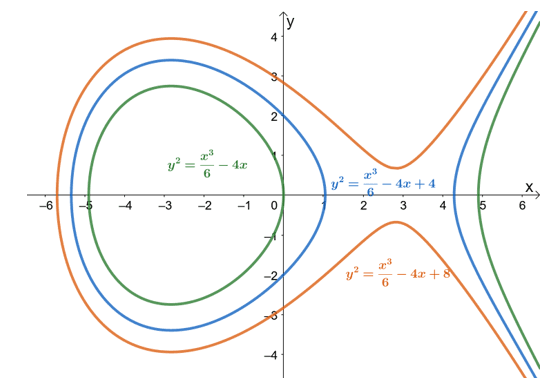
The graph shown above shows three equations that will satisfy the differential equation. In the next example, we’ll see what happens when we’re given an initial value for the differential equation.

Example 2

Solve the differential equation, $0.245\dfrac{dv}{dt} = 9.8v$, given that we have an initial value for the function: $v(0) = 36$.

Solution

This is an example of an initial value problem – when our differential equations come with enough initial conditions for us to find the value of the unknown constants. We can separate the variables with $v$ on the left-hand side of the equation.

 \begin{aligned}\dfrac{dv}{dt} &= \dfrac{9.8v}{0.245} \\ \dfrac{dv}{v} &= 40 \phantom{x}dt \\ \int \dfrac{dv}{v} &= \int 40 \phantom{x}dt \\\ln v &= 40t + C\end{aligned}

Now, let’s use the initial condition, $v(0) = 36$, and substitute these values into the equation to solve for $C$.

\begin{aligned} \ln 36 &= 40(0) + C\\C&= \ln 36\end{aligned}

Use this value to complete the solution for the initial-value problem: $\ln v = 40t + \ln 36$. Let’s rewrite this equation to only have $v$ on the left-hand side of the equation.

\begin{aligned} \ln v &= 40t + \ln 36\\ e^{\ln v} &= e^{40t + \ln 36}\\v &= e^{40t} e^{\ln 36}\\&= 36e^{40t}\end{aligned}

We call this solution, $v = 36e^{40t}$, a particular solution since this satisfies the differential equation with a given initial condition.

Practice Questions

1. Solve the differential equation, $3y \phantom{x}dy = (x^2 – 9) \phantom{x}dx$.
2. Solve the differential equation, $-5x^2 \phantom{x}dx = (4y^3 – 2y) \phantom{x}dy$.
3. Solve the differential equation, $\dfrac{dy}{dx} = \dfrac{x(e^{x^2} – 4)}{8y^2}$, given that we have an initial value for the function: $y(0) = 1$.
4. Solve the differential equation, $y^{\prime} = e^{x + 6y}$, given that we have an initial value for the function: $y(0) = 0$.

Answer Key

1. $y^2 = \dfrac{2x^3}{9} – 6x + C$
2. $x^3 = -\dfrac{3y^4}{5} + \dfrac{3y^2}{5} + C$
3. $\dfrac{8y^3}{3} = -2x^2 + \dfrac{1}{2}e^{x^2} + \dfrac{13}{6}$
4. $y = -\dfrac{1}{6} \ln(7 – 6e^x)$

The images/mathematical drawings are created with GeoGebra.