Disk Method – Definition, Formula, and Volume of Solids

One of the significant applications of integral calculus is its role in calculating the volume of a three-dimensional figure. Through different techniques such as the disk method, we now have the tools to approximate the volumes of these unique solids through calculus. Solids of revolutions and the methods of calculating their volumes are commonly used in engineering and manufacturing systems.

The disk method allows us to find the solids of the revolution’s volumes.  The disk method depends on revolving the curve with respect to the $\boldsymbol{x}$-axis.

In our discussion, you’ll learn what makes the disk method unique. We’ll also do a quick recap of what solids of revolution are. We’ll also show you the conditions and steps we need to remember when implementing the disk method to obtain the solids of the revolution’s volume.

What is the disk method?

The disk method allows us to calculate the volume of solids of revolution using cylindrical disks. Here’s a mental exercise: imagine a rectangle with one side adjacent to an axis. Revolve the rectangle around (at $360^{\circ}$) and complete one full revolution. The resulting figure is actually a right cylinder. This cylinder is considered a solid revolution and the line we used as a reference to revolve it is called the axis of revolution.

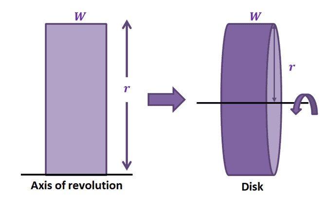
In fact, the volume of the resulting cylinder is equal to $\pi r^2 W$. We’ll break this down as this formula will later come in handy:

\begin{aligned}\binom{\text{Volume of}}{\text{Resulting Disk}} &=\binom{\text{Area of}}{\text{ Disk}}\times \binom{\text{Width of}}{\text{ Disk}} \\&= (\pi r^2) \cdot W\end{aligned}

Let’s extend this idea to revolving cross-sections about a given axis. This means that $y = f(x)$’ s area under its curve from $x =a$ to $x =b$ can be rotated about the $x$-axis. When that happens, the common result is having a solid revolution where the resulting cross-section is a circular disk that is perpendicular to the $\boldsymbol{x}$-axis.

Disk method definition

The disk method makes use of a cylindrical disk to estimate the volume of the solid of the revolution formed. Here’s how the disk of the solid of revolution formed by rotating the region under the curve of $f(x)$ and about the $x$-axis. We can rotate the region under the curve of $f(x)$ by reflecting its curve parallel to the axis of rotation. The disk is cylindrical in shape, so one slice of the disk (see image below) would have a volume of $\boldsymbol{\pi r^2 \Delta x}$, where $\boldsymbol{\approx f(x_i)}$.

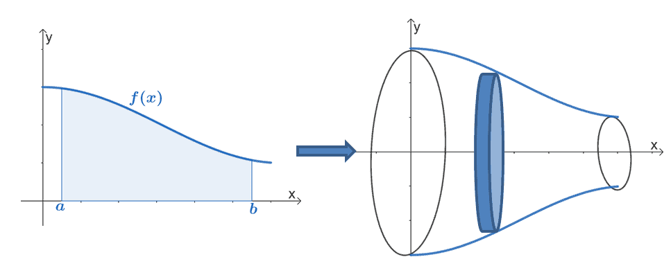
Let’s say we divide the interval, $[a, b]$ into $n$ disks, we can estimate the solid of revolution’s volume as shown below.

\begin{aligned}\sum_{i = 0}^{n -1} \pi [f(x_i)]^2 \Delta x\end{aligned}

When the function, $f(x)$, is above the $x$-axis and continuous throughout the interval fo $[a, b]$. We can estimate the solid of revolution’s volume through the disk method using the formula shown below:

\begin{aligned}V&= \lim_{\Delta x \rightarrow 0} \sum_{i = 0}^{n -1} \pi[f(x_i)]^2 \Delta x\\&= \int_{a}^{b} \pi[f(x)]^2 \phantom dx\end{aligned}

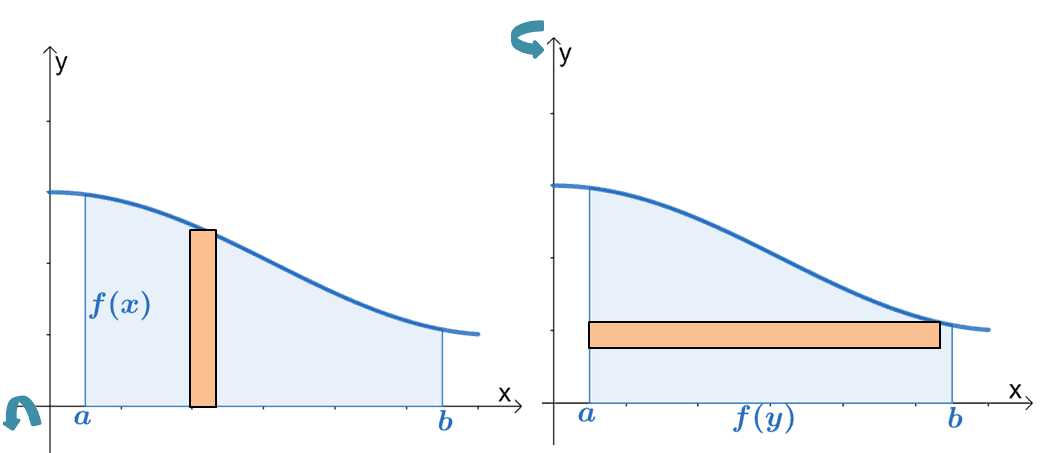
There are instances, however, when we need to rotate a curve with respect to the $y$-axis. We can also revolve the region about the $y$-axis. The formula will be similar except for the fact that we’re working with a function in terms of $y$ and with respect to $dy$.

\begin{aligned}V&= \lim_{\Delta y \rightarrow 0} \sum_{i = 0}^{n -1} \pi[f(y_i)]^2 \Delta y\\&= \int_{a}^{b} \pi[f(y)]^2 \phantom dy\end{aligned}

These are the two equations representing the solid’s volume. We only depend on orientation of the rotation. In the next section, we’ll be breaking down the steps of the disk method and learn how to apply these steps to find volume of solid of revolution.

How to use the disk method?

Use the guidelines below when using the disk method to estimate the solids of revolution’s volume:

• Identify the axis of revolution and set up the appropriate definite integral for the volume.
• When needed, sketch the disk and the solid of revolution using $\Delta x$ as the width and $x$ as the radius. When rotated vertically, use the values of $\Delta y$ and $y$ instead.
• Apply appropriate integral properties and techniques to find the antiderivative of $f(x)$ or $f(y)$.
• Evaluate the definite integral. Make sure that the volume is positive.

Why don’t we go ahead and refresh what we know of the two possible volumes? We’ve included a summary of the formulas for the disk method so you can easily access them when working on the problems that follow.

Disk method formula

Here’s a summary of the disk method formula highlighting how we calculate the volume depending on the axis of revolution.

Apply this formula to calculate the volume of a region, $f(x)$ or $f(y)$, about the horizontal or vertical axes, respectively.

Let’s try to find the volume of the solid formed by rotating $y = -x -1$ about the $x$-axis from $x = 0$ to $x = 2$.

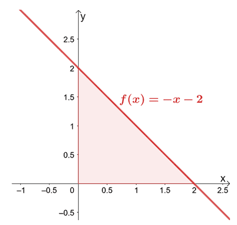
Since we’re rotating over the $x$-axis we’re integrating $f(x)$ from $x =0$ to $x =2$.  We’ve included the result of rotating $y = -x -2$ over the horizontal axis to help you visualize the disk formed.

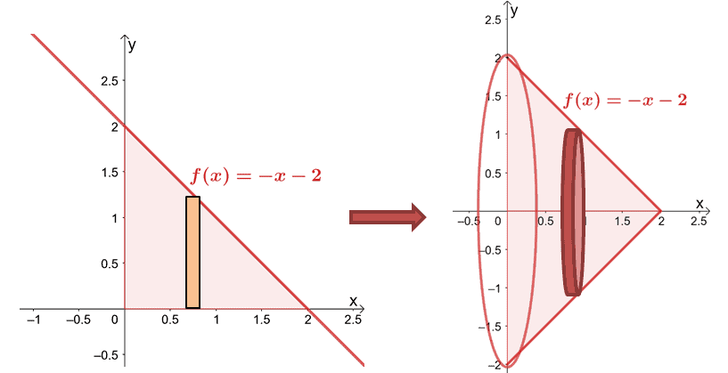
Let’s calculate the volume using the formula, $V = \pi\int_{a}^{b} [f(x)]^2 \phantom{x} dx$.

\begin{aligned}V &= \pi\int_{0}^{2} (-x -2)^2 \phantom{x} dx \\&= \pi \int_{0}^{2} (x^2 + 4x + 4)\phantom{x} dx\\&= \pi \left[\dfrac{x^3}{3} + \dfrac{4x^2}{2} + 4x \right ]_{0}^{2}\\&= \pi \left(\dfrac{2^3}{3}+ \dfrac{4\cdot 2^2}{2} + 4\cdot 2 \right )\\&= \dfrac{38}{3}\pi\end{aligned}        

This means that the solid’s volume is $\dfrac{38\pi}{3}$.

There are instances when it’s convenient to integrate an expression with respect to $x$ or with respect to $y$ so use your knowledge of the integration process to decide which would be a better option. Head over to the next section to work on more examples!

Example 1

Calculate the volume of the solid formed by revolving the region of the curve of $ f(x) =\sqrt{\sin x}$ about the $x$-axis and over the interval, $x = 0$ and $x = \pi$.

Solution

We’ll sketch the curve of $f(x) = \sqrt{\sin x}$ then show how the area under the curve would appear once rotated over the horizontal axis.

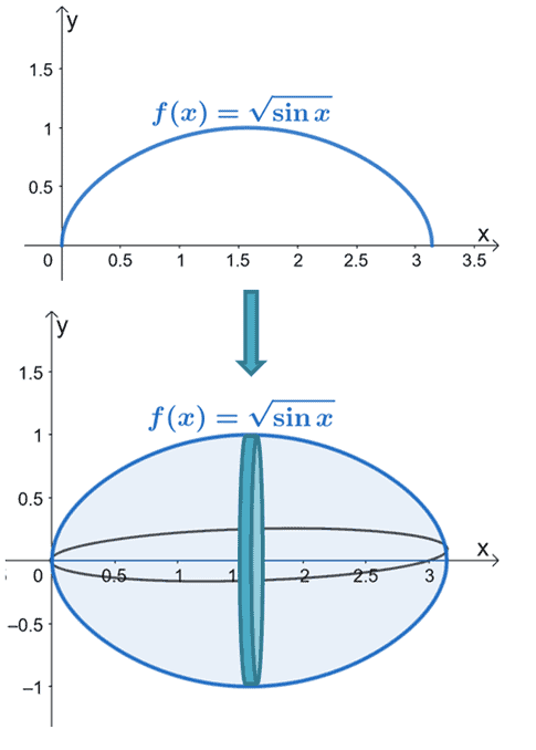
Find the volume of $f(x)$ by using the formula for the disk method with respect to the horizontal axis.

\begin{aligned}V&= \pi\int_{0}^{\pi} (\sqrt{\sin x})^2 \phantom{x}dx\\&= \pi \int_{0}^{\pi} \sin x \phantom{x}dx\end{aligned}

Integrate the expression by using the antiderivative formula, $\int \sin x \phantom{x}dx = – \cos x+ C$. Evaluate the resulting antiderivative at $x = 0$ and $x =\pi$.

\begin{aligned}\pi \int_{0}^{\pi} \sin x \phantom{x}dx &=\pi \left[ -\cos x\right]_{0}^{\pi}\\ &=\pi[ (-\cos \pi) – (-\cos 0)]\\&= \pi(1 + 1)\\&= 2\pi \end{aligned}

This means that the volume of the solid formed is equal to $2\pi$.

Example 2

Find the volume of the solid formed by revolving the region of the curve of $ y = 27x^3$ about the $y$-axis and over the interval, $y = 0$ and $y = 4$.

Solution

Since we’re revolving the curve over the vertical axis, let’s find the expression of the curve in terms of $y$.

\begin{aligned} y&= 27x^3\\ \sqrt[3]{y} &= \sqrt[3]{27x^3}\\ \sqrt[3]{y}  &= 3x\\x &= \dfrac{1}{3}y^{\frac{1}{3}}\end{aligned}

Let’s sketch the region under the curve of $x = \dfrac{1}{3}y^{\frac{1}{3}}$ then rotate the region over the $y$-axis from $y =0$ to $y =4$.

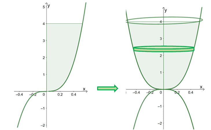
Here’s the solid formed by rotating the curve over the $y$-axis. We’ve included a slice of the disk to highlight how the rotation’s orientation affects the disk’s volume as well. We’ll use the formula for the disk method with respect to the vertical axis to find the solid’s volume.

\begin{aligned}V&= \int_{a}^{b} f(y) \phantom{x}dy\\ &=\pi\int_{0}^{4 } \left(\dfrac{1}{3}y^{\frac{1}{3}}\right)^2 \phantom{x}dy\\ &=\pi\int_{0}^{4 } \dfrac{1}{9}y^{\frac{2}{3}} \phantom{x}dy \\ &=\dfrac{\pi}{9}\int_{0}^{4 } y^{\frac{2}{3}} \phantom{x}dy \end{aligned}

Apply the power rule, $\int x^n \phantom{x}dx = \dfrac{x^{n + 1}}{n + 1} +C$, to integrate the expression then evaluate the antiderivative at $y =0$ and $y =4$.

\begin{aligned}\dfrac{\pi}{9}\int_{0}^{4 } y^{\frac{2}{3}} \phantom{x}dy &= \dfrac{\pi}{9}\left[\dfrac{y^{\frac{2}{3} +1}}{\dfrac{2}{3} +1} \right ]_{0}^{4}\\ &= \dfrac{\pi}{9}\cdot \dfrac{3}{5}\left[y^{\frac{2}{3} + 1}\right]_{0}^{4}\\&= \dfrac{\pi}{15} \left(4^{\frac{2}{3}} + 4^1\right )\\&\approx 1.366   \end{aligned}

This means that the volume of the solid obtained by rotating $ y = 27x^3$ over the $y$-axis is approximately 2.11101798104.

Practice Questions

1. Calculate the volume of the solid formed by revolving the region of the curve of $ f(x) =\sqrt{\cos x}$ about the $x$-axis and over the interval, $x = 0$ and $x = \dfrac{\pi}{2}$.

2. Calculate the volume of the solid formed by revolving the region of the curve of $ f(x) =\sqrt{4x }$ about the $x$-axis and over the interval, $x = 0$ and $x = 4$.

3. Calculate the volume of the solid formed by revolving the region of the curve of $ f(x) =\dfrac{1}{x}$ about the $x$-axis and over the interval, $x = 1$ and $x = 6$.

4. Find the volume of the solid formed by revolving the region of the curve of $ x = 3\sqrt{y}$ about the $y$-axis and over the interval, $y = 0$ and $y = 16$.

5. Find the volume of the solid formed by revolving the region of the curve of $ y = \ln x$ about the $y$-axis and over the interval, $y = 1$ and $y = 2$.

6. Find the volume of the solid formed by revolving the region of the curve of $x = 2y^2 – 4y + 1$ about the $y$-axis and over the interval, $y = 4$ and $y = 8$.

Answer Key

1. $\pi$
2. $8 \pi$
3. $\dfrac{5\pi}{6}$
4. $128 \pi$
5. $(e^2 – e)\pi$
6. $\dfrac{620\pi}{3}$

Images/mathematical drawings are created with GeoGebra.