Least Squares – Explanation and Examples

Least squares is a method of finding the best line to approximate a set of data.

In particular, least squares seek to minimize the square of the difference between each data point and the predicted value.

This section covers:

• What is the Least Squares Method?
• Least Squares Method Definition
• Least Squares Method Formula

What Is the Least Squares Method?

The least squares method seeks to find a line that best approximates a set of data. In this case, “best” means a line where the sum of the squares of the differences between the predicted and actual values is minimized.

Why does this use the squares? Why not just find the sum of the differences between the predicted and actual values in these problems?

In some cases, the predicted value will be more than the actual value, and in some cases, it will be less than the actual value. In either event, however, the predicted value is inaccurate.

Just finding the difference, though, will yield a mix of positive and negative values. Thus, just adding these up would not give a good reflection of the actual displacement between the two values.

The squares, however, will always be positive. Therefore, adding these together will give a better idea of the accuracy of the line of best fit.

The least squares method uses a specific formula to find the line, $y=mx+b$, that minimizes this sum.

Least Squares Method Definition

The least squares method is a method for finding a line to approximate a set of data that minimizes the sum of the squares of the differences between predicted and actual values.

This line has the form $y=mx+b$ where $m$ and $b$ are calculated using the given data set’s $x$ and $y$ values.

Least Squares Method Formula

The goal of the least squares method is to find a line with the equation $y=mx+b$ that best approximates the data. This is sometimes called the line of best fit.

Here, “best” means that the sum of the squares of the differences between the actual data points and their predicted values on the line is minimized. Hence, the name “least squares.”

This least squares line for a set of data with points $(x_1, y_1)$, … , $(x_n, y_n)$ is $y=mx+b$ where $m$ and $b$ are as follows.

$m=\frac{n[(x_1y_1)+ … +(x_ny_n)]-[(x_1 + … + x_n)(y_1 + … + y_n)]}{(x_1^2 + … + x_n^2)-(x_1 + … + x_n)^2}$.

This is equivalent to:

$m=\frac{ n\sum\limits_{i=1}^n xy – [(\sum\limits_{i=1}^n x)(\sum\limits_{i=1}^n y)]}{n\sum\limits_{i=1}^n x^2 – (\sum\limits_{i=1}^n x)^2}$.

and

$b=\frac{\sum\limits_{i=1}^n y – [(m)(\sum\limits_{i=1}^n x)]}{n}$.

Examples

This section covers common examples of problems involving least squares and their step-by-step solutions.

Example 1

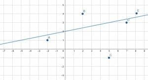
What is the predicted value for $x=5$?

Solution

The predicted value for $x=5$ is the point on the given line where $x=5$. Note that this may be different from the actual value at $x=5$.

In this case, the actual value when $x=5$ is $y=-1$.

But the prediction line has a different value of $y=3$.

Example 2

Find the total of the squares of the difference between the actual values and the predicted values.

Solution

First, it is helpful to find the equation of the line. This will help to find the predicted values.

Note that the line passes through $(0, 2)$ and $(5, 3)$. This means that the slope of the line is $m=\frac{3-2}{5-0}=\frac{1}{5}$. Its y-intercept is $2$, so the equation is $y=\frac{1}{5}x+2$.

The given values are $(-2, 1), (2, 4), (5, -1), (7, 3),$ and $(8, 4)$.

Plugging the $x$ values into the equation gives:

$y=\frac{1}{5}(-2)+2=\frac{8}{5}$.

$y=\frac{1}{5}(2)+2-\frac{12}{5}$.

The value for $5$ is known to be $3$.

$y=\frac{1}{5}(7)+2=\frac{17}{5}$.

$y=\frac{1}{5}(8)+2=\frac{18}{5}$.

The difference between the predicted and actual values for $x=-2$ is $\frac{8}{5}-1=\frac{3}{5}$. Then, squaring that gives $\frac{9}{25}$.

The difference between the predicted and actual values for $x=2$ is $\frac{12}{5}-4=-\frac{8}{5}$. Then, squaring that gives $\frac{64}{25}$.

The difference between the predicted and actual values for $x=5$ is $3+1=4$. Squaring that value gives $16$.

The difference between the predicted and actual values for $x=7$ is $\frac{17}{5}-3=\frac{2}{5}$. Then, squaring that gives $\frac{4}{25}$.

The difference between the predicted and actual values for $x=8$ is $\frac{18}{5}-4=-\frac{2}{5}$. Then, squaring that gives $\frac{4}{25}$.

The total is therefore: $\frac{9}{25}+\frac{64}{25}+\frac{400}{25}+\frac{4}{25}+\frac{4}{25}=\frac{481}{25}$. This is equal to $19\frac{6}{25}$.

Example 3

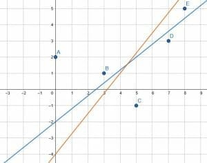
Find the better of the two lines by comparing the total of the squares of the differences between the actual and predicted values.

Solution

The blue line is the better of these lines because the total of the square of the differences between the actual and predicted values is smaller.

First, find the actual values for the five points.

$A=(0, 2)$

$B=(3, 1)$

$C=(5, -1)$

$D=(7, 3)$

$E=(8, 5)$.

Then, find the equation of the two lines.

Note that the blue one passes through $(0, -2)$ and $(4, 1)$. Therefore, its slope is $m=\frac{4}{5}$, and its equation is $y=\frac{4}{5}x-2$.

Similarly, the orange line passes through $(0, -4)$and $(4, 1)$. Thus, its slope is $m=\frac{5}{4}$, and its equation is $y=\frac{5}{4}x-4$.

Now, it is required to find the predicted value for each equation. To do this, plug the $x$ values from the five points into each equation and solve.

Doing this shows that the predicted values for the blue line are $(0, -2), (3, \frac{2}{5}), (5, 2), (7, \frac{18}{5}),$ and $(8, \frac{22}{5})$.

Using a similar process, the predicted values for the orange line are $(0, -4), (3, -\frac{1}{4}), (5, \frac{9}{4}), (7, \frac{19}{4}),$ and $(8, 6)$.

Next, find the difference between the actual value and the predicted value for each line. Then, square these differences and total them for the respective lines.

Blue line:

Differences are $4, \frac{3}{5}, 3, \frac{3}{5},$ and $\frac{3}{5}$.

These values squared are $16, \frac{9}{25}, 9, \frac{9}{25},$ and $\frac{9}{25}$.

Then, totaling these squares yields $\frac{652}{25}$ or $26\frac{2}{25}$.

Orange line:

Differences are $6, \frac{5}{4}, \frac{13}{4}, \frac{7}{4},$ and $1$.

These values squared are $36, \frac{25}{16}, \frac{169}{16}, \frac{49}{26},$ and $1$.

Then, totaling these squares yields $\frac{835}{16}$ or $52\frac{3}{16}$.

Since the sum for the blue line, $26\frac{2}{25}$, is less than the sum for the orange line, $52\frac{3}{16}$, it is a better approximation of the data.

Example 4

Find the least squares line for the data given below.

(1, 5), (9, -2), (5, 2), (3, 4)

Solution

Here, it is not necessary to plot the points. It is just required to find the sums from the slope and intercept equations.

Recall that:

$m=\frac{n \sum\limits_{i=1}^n xy – [(\sum\limits_{i=1}^n x)(\sum\limits_{i=1}^n y)]}{n\sum\limits_{i=1}^n x^2 – (\sum\limits_{i=1}^n x)^2}$.

and

$b=\frac{\sum\limits_{i=1}^n y – [(m)(\sum\limits_{i=1}^n x)]}{n}$.

This means it is required to find $\sum\limits_{i=1}^n xy$, $\sum\limits_{i=1}^n x$, $\sum\limits_{i=1}^n x^2$, and $\sum\limits_{i=1}^n y$. Then, plug these into the equations for $m$ and $b$.

$\sum\limits_{i=1}^n xy=(1\times5)+(9\times -2)+(5\times2)+(3\times4)=5-18+10+12=9$

$\sum \limits_{i=1}^n x=1+9+5+3=18$

$\sum\limits_{i=1}^n x^2=1^2+9^2+5^2+3^2=1+81+25+9=116$

$\sum\limits_{i=1}^n y=5-2+2+4=9$.

Now, plugging these into the formulas yields:

$m=\frac{4(9)-(18)(9)}{4(116)-18^2}=\frac{36-162}{464-324}=\frac{-126}{140}=\frac{9}{10}=0.9$.

$b=\frac{9-[-0.9\times 18]}{4}=\frac{9+16.2}{4}=\frac{25.2}{4}=6.3$.

Therefore, the equation for the line is $y=-0.9x+6.3$.

Example 5

(1, 4), (3, 7), (4, 6), (6, 8)

Find the least squares line for the data given and use it to predict the $y$ value when $x=10$.

Solution

As before, find the relevant sums for the equations for $m$ and $b$. Then, substitute $x=10$ into the equation for the line of best fit.

$\sum\limits_{i=1}^n xy=(1\times4)+(3 \times7)+(4\times6)+(6\times8)=4+21+24+48=97$

$\sum \limits_{i=1}^n x=1+3+4+6=14$

$\sum\limits_{i=1}^n x^2=1+9+16+36=62$

$\sum\limits_{i=1}^n y=4+7+6+8=25$.

Now, plugging these into the formulas yields:

$m=\frac{4(97)-(14)(25)}{4(62)-196}=\frac{388-350}{248-196}=\frac{38}{52}=\frac{19}{26}$.

$b=\frac{25-[\frac{19}{26}\times 14]}{4}=\frac{48}{13}$.

Therefore, the equation for the line of best fit is $y=\frac{19}{26}x+\frac{48}{13}$.

To find the approximation for $x=10$, plug this value into that equation. This yields:

$y=\frac{19}{26}(10)+\frac{48}{13}=\frac{95}{13}+\frac{48}{13}=\frac{143}{13}=11$.

Thus, the estimate for $y$ when $x=10$ is $11$.

Practice Problems

1. The line of best fit for a set of data is $y={6}{5}x-7$. If the actual value for $x=10$ is 8, what is the difference between the actual and predicted values?
2. Consider the data set $(-4, 5), (-1, 10), (6, 15), (7, 16)$ and the line $y=x+9$.
   What is the sum of the squares of the differences between the actual and predicted values?
3. Based on the previous problem, what does it mean if the sum of the squares of the differences between the actual and predicted values is $0$?
4. Find the equation of the least squares line for the following data set:
   $(0, -3), (1, -2), (4, -1), (5, 4)$.
5. Find the least square line equation for the following data set and use it to predict $x=10$.
6. $(-1, -4), (0, 3), (1, 4), (2, 6)$.

Answer Key

1. $3$
2. $4$
3. If the sum of the squares of the differences is $0$, this means that the difference between the actual and predicted values is $0$ for all $x$ values. Therefore, all of the data points lie on a line. However, this does not mean that all of the points would continue to fall exactly on that line if more points were collected.
4. $y=\frac{19}{17}x-\frac{56}{17}$
5. The equation is $y=3.1x+0.7$, which predicts $y=31.7$ when $x=10$.

Images/mathematical drawings are created with GeoGebra.