JUMP TO TOPIC
Linear Programming Calculator + Online Solver With Free Steps
Linear Programming Calculator is a free online calculator that provides the best optimal solution for the given mathematical model.
This online calculator solves the problem of finding the correct solution or optimized output of the desired mathematical models by providing a quick, reliable, and accurate solution.
It just requires the user to enter the objective function along with the system of linear constraints and the solution will be on their screens just in a matter of seconds. The Linear Programming Calculator is the most efficient tool for linear optimization and can be used to solve complex and time-consuming problems and models effectively and logically.

What Is the Linear Programming Calculator?
The Linear Programming Calculator is an online calculator that can be used for the linear optimization of various mathematical models.
It is a convenient and user-friendly tool with an easy-to-use interface that helps the user to find the exact and optimized solution for the provided constraints faster than any other mathematical technique applied manually.
The Linear Programming Calculator helps the user to avoid the long mathematical calculations and get the desired answer just by clicking one button.
The calculator can solve problems containing a maximum of nine different variables not more than that. It requires “,” as a separator for multiple constraints in a single box.
Let’s find out more about the calculator and how it works.
How To Use a Linear Programming Calculator?
You can use the Linear Programming Calculator by entering the objective function and specifying the constraints. Once you are done entering all the inputs you just have to press the submit button and a detailed solution will be displayed on the screen just in seconds.
Following are the detailed stepwise guidelines to find out the best possible solution for the given objective function with specified constraints. Follow these simple steps and find out the maxima and minima of the functions.
Step 1
Consider your desired objective function and specify its constraints.
Step 2
Now, enter the objective function in the tab specified as Objective Function.
Step 3
After adding the objective function, input the conditions of all constraints in the tab named Subject. The calculator can take a maximum of nine constraints and has more tabs for it under the name More Constraints. To add multiple constraints in a single block, you have to use “,” as a separator.
Step 4
Once you are done filling all the input fields, select the optimization category from the Optimize drop-down menu. There are three options you can select to find the maxima of the objective function, minima of the objective function or you can select both.
The options in the drop-down menu are given as:
- Max
- Min
- Max/Min
Step 5
After that, press the Submit button and the optimal solution along with graphs will be displayed in the result window.
Make sure not to add more than nine constraints in the calculator, otherwise it will fail to produce the desired results.
Step 6
You can view the result window below the calculator layout. The Result window contains the following blocks:
Input Interpretation
This block shows the input entered by the user and how it has been interpreted by the calculator. This block helps the user to figure out if there were any mistakes in the input data.
Global Maximum
This block shows the calculated global maxima of the given objective function. Global maxima are the overall largest value of the objective function.
Global Minimum
This block displays the global minima of the given objective function. Global minima are the overall smallest value of the given function with the specified constraints.
3D Plot
This block displays the 3D interpretation of the objective function. It also specifies the maxima and minima points on the 3D plot.
Contour Plot
The contour plot is a 2D representation of the global maxima and global minima of the objective function on the graph.
How Does the Linear Programming Calculator Work?
The Linear Programming Calculator works by computing the best optimal solution of the objective function using the technique of Linear programming, which is also called Linear optimization.
Mathematical optimization is the technique used to find the best possible solution to a mathematical model such as finding the maximum profit or analyzing the size of the cost of a project, etc. It is the type of linear programming that helps to optimize the linear function provided that given constraints are valid.
To understand more about the working of the Linear Programming Calculator, let’s discuss some of the important concepts involved.
What Is Linear Programming (LP)?
Linear Programming is the mathematical programming technique that tends to follow the best optimal solution of a mathematical model under specified conditions which are called constraints. It takes various inequalities applied to a certain mathematical model and finds the optimum solution.
Linear Programming is only subjected to linear equality and inequality constraints. It is only applicable to linear functions that are the first-order functions. The linear function is usually represented by a straight line and the standard form is y = ax + b.
In linear programming, there are three components: decision variables, objective function, and constraints. The usual form of a linear program is given as follows:
The first step is to specify the decision variable that is an unknown element in the problem.
decision variable = x
Then, decide whether the optimization required is the maximum value or the minimum value.
The next step is to write the objective function that can be maximized or minimized. The objective function can be defined as:
\[ X \to C^T \times X \]
Where C is the vector.
Finally, you need to describe the constraints that can be in the form of equalities or inequalities and they must be specified for the given decision variables.
The constraints for the objective function can be defined as:
\[ AX \leq B \]
\[ X \geq 0 \]
Where A and B are the vectors. Therefore, linear programming is an effective technique for the optimization of various mathematical models.
Thus, the Linear Programming Calculator uses the linear programming process to solve the problems in seconds.
Due to its effectiveness, it can be utilized in various fields of study. Mathematicians and businessmen use it widely, and it is a very useful tool for engineers to help them solve complex mathematical models that are formed for various designing, planning, and programming purposes.
Representing Linear Programs
A linear program can be represented in various forms. First, it requires the identification of the maximization or minimization of the objective function and then the constraints. The constraints can be either in the form of inequalities $( \leq , \geq )$ or equality ( = ).
A linear program can have decision variables represented as $ x_1, x_2, x_3, …….., x_n $.
Therefore, the general form of a Linear Program is given as:
Minimize or Maximize:
\[ y = c_o + c_1x_1 + c_2x_2 + …. + c_nx_n \]
Subject to:
\[ a_1i x_1+ a_2ix_2 + a_3ix_3 +……. + a_nix_n = b_i \]
\[ a_1ix_1 + a_2ix_2 + a_3ix_3 +……. + a_nix_n \leq b_i \]
\[ a_1ix_1+ a_2ix_1 + a_3ix_2 +……. + a_nix_n \geq b_i \]
Where i = 1,2,3,……..,m.
\[ x_k \geq 0 \]
\[ x_k < 0 \]
\[ x_k > 0 \]
Where k = 1,2,3,……..,m.
Here $x_k$ is the decision variable and $a_in$, $b_i$, and $c_i$ are the coefficients of objective function.
Solved Examples
Let’s discuss some examples of linear optimization of the mathematical problems using the Linear Programming Calculator.
Example 1
Maximize and minimize the objective function given as:
\[ 50x_1 + 40x_2 \]
The constraints for the above-mentioned objective function are given as:
\[3x_1 + 1x_2 <= 2700 \]
\[ 6x_1 + 4x_2 >= 600 \]
\[ 5x_1 + 5x_2 = 600 \]
\[ x_1 \geq 0 \]
\[ x_2 \geq 0 \]
Use the calculator to optimize the given function.
Solution
Follow the steps mentioned below:
Step 1
Select the max/min option from the Optimize drop-down menu.
Step 2
Input the objective function and the functional constraints in the specified blocks.
Step 3
Now click the submit button to view the results.
The Global maximum of the function is given as:
\[ max( 50x_1 + 40x_2 )_{at ( x_1, x_2 )} = (120, 0 ) \]
The Global minimum of the function is given as:
\[ min ( 50x_1 + 40x_2 )_{at ( x_1, x_2 )} = (60, 60 ) \]
The 3D plot is shown in Figure 1:
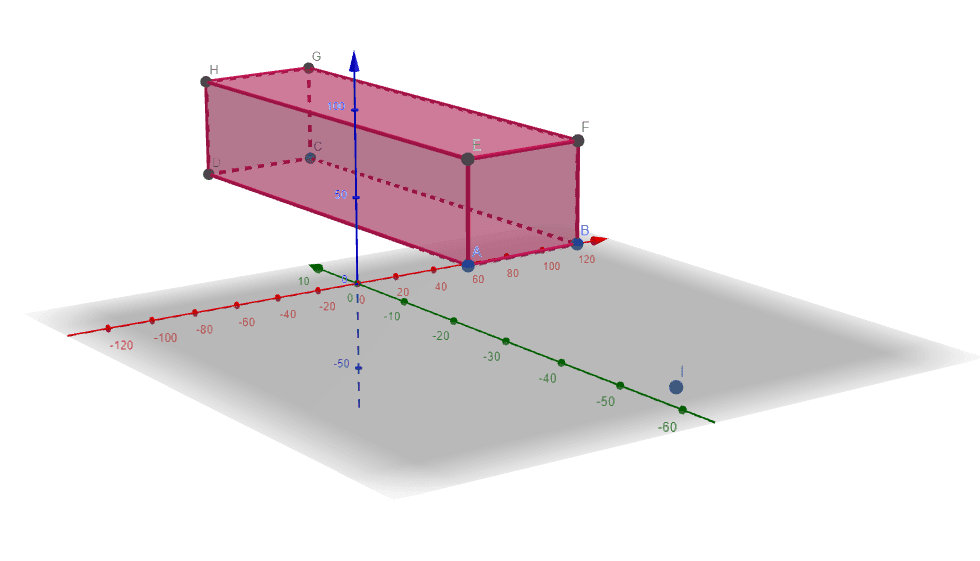
Figure 1
The contour plot is given in Figure 2 below:
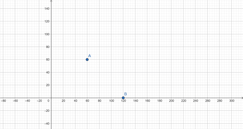
Figure 2
Example 2
A diet plan chalked by the dietitian contains three types of nutrients from two types of food categories. The nutritional contents under study include proteins, vitamins, and starch. Let the two food categories be $x_1$ and $x_2$.
A specific amount of each nutrient must be consumed each day. The nutritional content of proteins, vitamins, and starch in food $x_1$ is 2, 5, and 7, respectively. For food category $x_2$ the nutritional contents of proteins, vitamins, and starch are 3,6, and, 8, respectively.
The requirement per day of each nutrient is 8, 15, and 7, respectively.
The cost of each category is $2$ per $kg$. Determine the objective function and constraints to find out how much food must be consumed per day to minimize the cost.
Solution
The decision variable are $x_1$ and $x_2$.
The objective function is given as:
\[ y = 2x_1 + 2x_2 \]
The various constraints for the given objective function analyzed from the data given above are:
\[ x_1 \geq 0 \]
\[ x_2 \geq 0 \]
\[ 2x_1 + 3x_2 > 8 \]
\[ 5x_1 + 6x_2 > 15 \]
\[ 7x_1 + 8x_2 > 7 \]
All the constraints are non-negative as the amount of food cannot be negative.
Input all the data in the calculator and press the submit button.
Following results are obtained:
Local Minimum
\[ min( 2x_1 + 2x_2 ) = (0, 2.67)
3D Plot
The 3D representation is shown in figure 3 below:
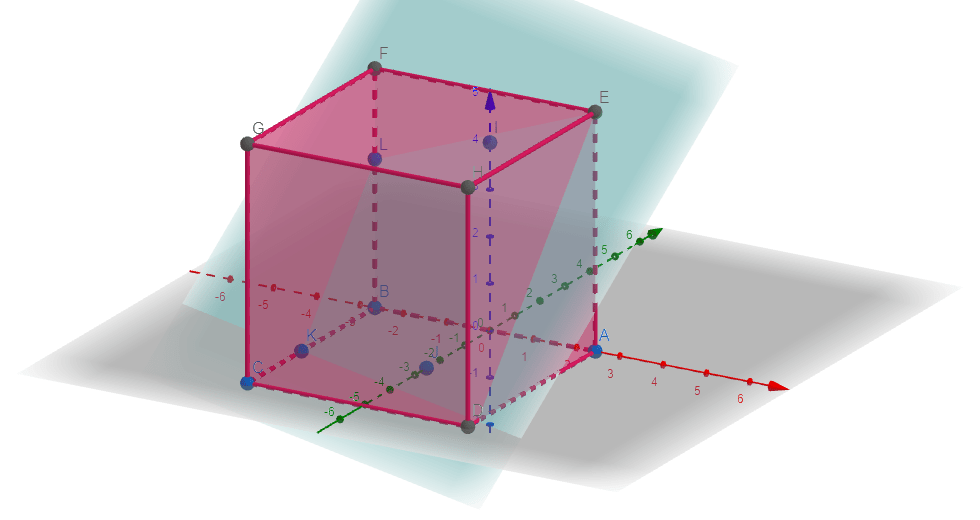
Figure 3
Contour Plot
The contour plot is shown in Figure 4:
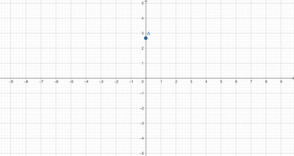
Figure 4
All the Mathematical Images/Graphs are created using GeoGebra.