Curve sketching – Properties, Steps, and Examples

Curve sketching shows us how we can understand and predict the behavior of the function based on its first and second derivatives. Functions and their graphs are important not only in math but in other fields and applications as well. Whenever we need to observe quantities and how they relate to each other, we need functions to model their relationship.  This is why it’s important to know how the functions’ graphs were formed.

Curve sketching the process of predicting the function’s graph given its expression. It is also an application of our knowledge on first and second derivative tests.

Knowing how to graph a function will be most helpful when you don’t have graphing utilities available. Mastering curve sketching will also make you understand and appreciate the math behind these graphing utilities. Aside from this practical reason, knowing how to sketch curves will also strengthen our understanding of first and second derivative tests.   

In our discussion, we’ll show we can apply the two derivative tests to predict the shape of a given function’s graph. Make sure to review your notes on the first and second derivatives. When you’re ready, let’s go ahead and dive right into the process of sketching a function’s curve!

How to sketch a curve?

Curve sketching, as we have mentioned, is an important skill to learn in math that uses different precalculus and differential calculus topics we’ve learned in the past.

Here’s a graph of $y  =x^3 -3x$ and we’ve included the important components we need to graph the given function.

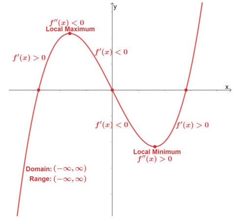
We can predict the function’s behavior and eventually be able to sketch their curves by knowing the intervals where the function is increasing, decreasing, concaving upward, and concaving downward. Use the different properties of the function such as its domain, asymptotes, and intercepts to be able to sketch the function’s curve more accurately.

In this section, we’ll discuss the important components you’ll need and we’ll include a quick refresher on the concept and theory used for each step.

Finding the intercepts of the graph:

Whenever possible, determine the $x$ and $y$-intercepts so that we can use them as additional guide points once we graph the function’s curve.

• Find the function’s $x$-intercept by equating $f(x)$ to $0$.

\begin{aligned}x_{\text{int}}: f(x) &= 0\end{aligned}

• Substitute $x= 0$ into $f(x)$ to find the $y$-intercepts of $f(x)$.

\begin{aligned}y_{\text{int}} &= f(0) \end{aligned}

Finding the function’s asymptotes:

Recall that one function may have a vertical asymptote, horizontal asymptote, or an oblique asymptote.

• Find the vertical asymptotes of the function by finding the restricted values from its domain. These are usually values of $x$ that may return a rational function’s denominator to zero or may return a negative value inside a radical expression.
• Determine the horizontal asymptote by finding the values of $\boldsymbol{\lim_{\infty} f(x)}$. If the degree of the denominator is larger, find the horizontal asymptote using our precalculus knowledge as well.
• When given a rational function, double-check if the function has an oblique asymptote. When the numerator’s degree is larger, find its oblique asymptote (if it exists) by evaluating $\boldsymbol{\lim_{x\rightarrow \infty} f(x)}$, where $f(x)$ is rewritten as a sum of a linear and a rational function.

Keep in mind that there are functions such as the polynomial functions where it has no asymptotes at all.

Checking the symmetry of the function:

This is most helpful when the curve has multiple inflections and extreme values. When you can confirm the symmetry of the function, use it and reflect the function’s curve accordingly. This will definitely shorten the time need to sketch a function’s curve.

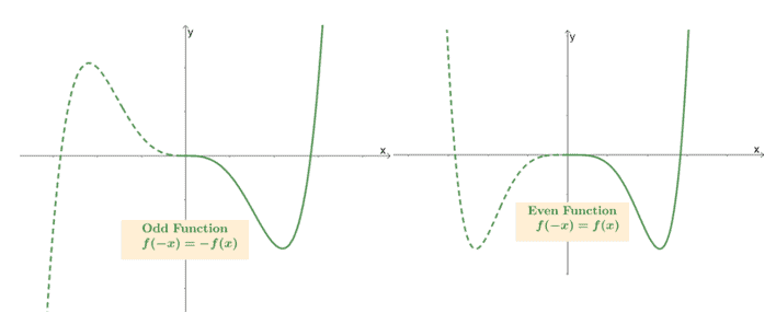
• When the function is odd, it satisfies the equation, $\boldsymbol{f(-x)= -f(x)}$. Once you have half of the curve’s domain already graphed, simply reflect the graph with respect to the origin.
• When the function is even, it has to satisfy the equation, $\boldsymbol{f(-x)= f(x)}$. Once you have half of the curve’s domain already graphed, simply reflect the graph along the $\boldsymbol{y}$-axis.

Learn more about even and odd functions here.

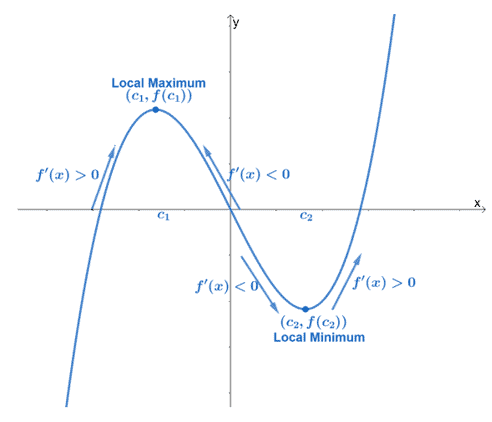
Finding the function’s critical points and extrema:

Find the relative maximum and minimum of the function by finding $f^{\prime}(x)$ and equating the expression to zero. Use what we know about the first derivative test to determine the function’s extrema:

• When $f^{\prime} (c)= 0$, $x= c$ is a critical point.
• If $f^{\prime}(x)$’s sign changes from $+$ to $-$ at $x =c$, the function has a local maximum at $c$.
• Similarly, when $f^{\prime}(x)$’s sign changes from $-$ to $+$ at $x =c$, the function has a local minimum at $c$.

We can also use the results from the rest of the intervals – make sure to keep in mind whether the function’s increasing or decreasing at the intervals we’ve tested.

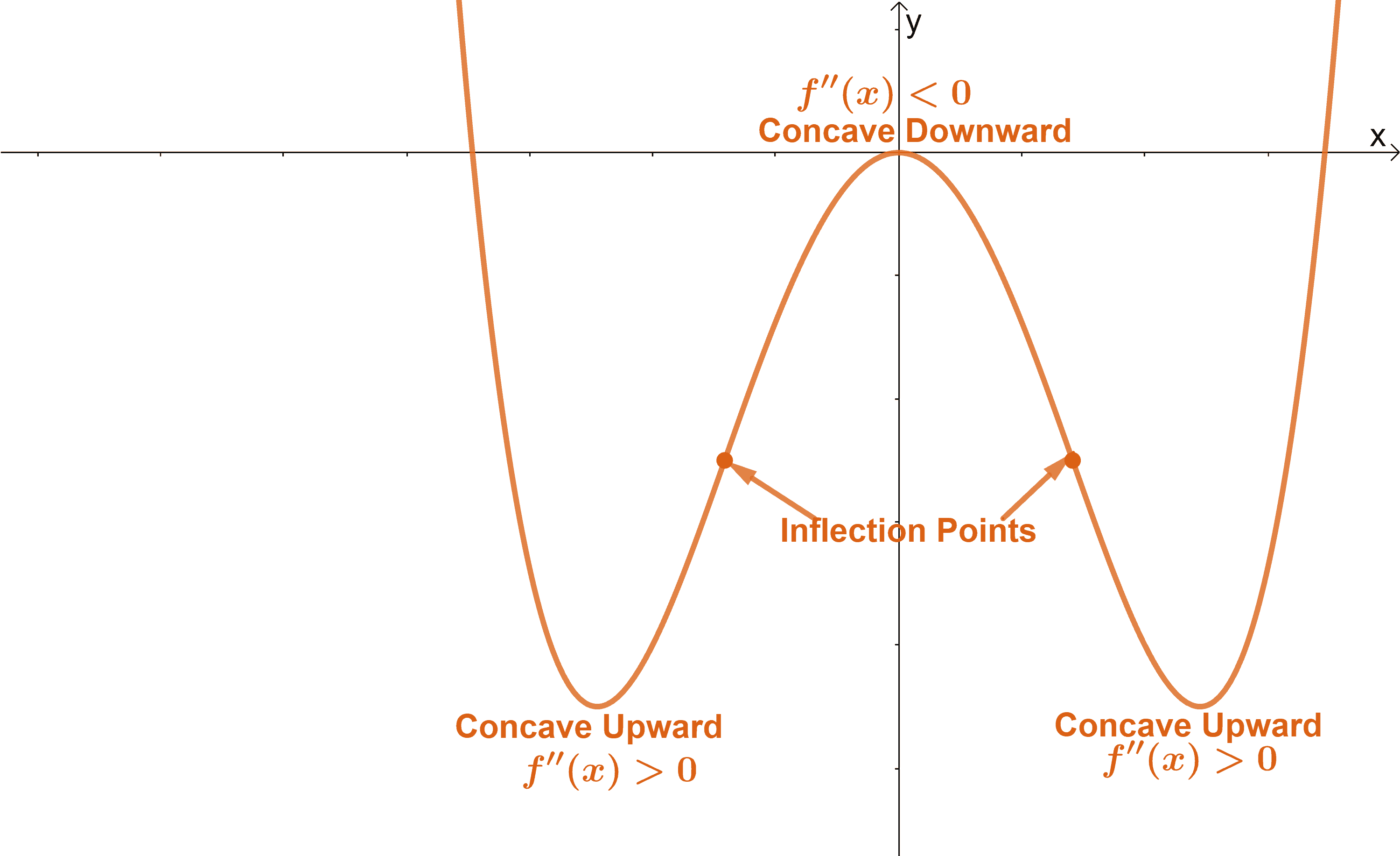
Determine the concavity of the graph and its points of inflection:

Let’s differentiate $f^{\prime}(x)$ one more time to find the expression for $f^{\prime\prime}(x)$. Once we have $f^{\prime\prime}(x)$, find the values where $f^{\prime\prime}(x)$ is either zero or undefined.

• When $\boldsymbol{f^{\prime\prime}(c) = 0}$, $x = c$ is a point of inflection.
• Use the values of $c$ to divide the domain of $f(x)$ into smaller intervals. Find a value between each interval and see if $\boldsymbol{f^{\prime\prime}(x)}$ is positive or negative.
• When $\boldsymbol{f^{\prime\prime}(x) >0}$, the function is concaving upwards at the interval. Meanwhile, when $\boldsymbol{f^{\prime\prime}(x) <0}$, the function is concaving downwards.

Once we have all the information, we can now sketch the function’s curve.

• Begin by graphing the function’s $x$ and $y$-intercepts.
• Include the function’s asymptotes and point of inflections.
• Take note of the local extrema and the intervals where the function is increasing or decreasing.
• Use the function’s concavity and points of inflection as well to help guide us in completing the curve.

Let’s use these pointers and apply them to sketch the graph of a given function.

How to apply the curve sketching steps to graph a given function?

Let’s say we want to graph $f(x) = \dfrac{1}{1 + x^2}$. We can use the steps we’ve just learned to sketch its curve. Begin by finding thse $x$ and $y$-intercepts of the function.

From this, we can see that $f(x)$ has no $\boldsymbol{x}$-intercepts and a $\boldsymbol{y}$-intercept at $\boldsymbol{(0, 1)}$. Let’s move on to the function’s asymptotes. Since $f(x)$’s denominator is equal to $x^2 +1$, this can never be equal to $0$, so the function has no restrictions for $x$. This means that $f(x)$ has no vertical asymptotes. Evaluate $\lim_{x \rightarrow \infty} f(x)$ to check for horizontal asymptotes.

\begin{aligned}\lim_{x \rightarrow\infty} f(x) &= \lim_{x \rightarrow\infty} \dfrac{1}{x^2 +1}\\&= \lim_{x \rightarrow\infty} \dfrac{1}{x^2 +1} \cdot \dfrac{\dfrac{1}{x^2}}{\dfrac{1}{x^2}}\\&=\lim_{x\rightarrow \infty} \dfrac{\dfrac{1}{x^2}}{1 + \dfrac{1}{x^2}}\\&= \dfrac{{\color{Teal}0}}{1 + {\color{Teal}0}},\phantom{x}{\color{Teal}\lim_{x \rightarrow \infty} \dfrac{1}{x^2}=0}\\&= 0\end{aligned}

Hence, $f(x)$ has a horizontal asymptote at $\boldsymbol{y= 0}$. Recall that a function can only have either a horizontal asymptote or an oblique asymptote but never both. For $f(x)$, we won’t have to check for oblique asymptotes anymore.

Now, let’s go ahead and check the function for symmetry by finding the expression of $f(-x)$.

\begin{aligned}f(-x)&= \dfrac{1}{1 + (-x)^2}\\&=\dfrac{1}{1 + x^2}\\&= f(x)\\&\Rightarrow\color{Teal}\text{Even Function}\end{aligned}

Since $f(-x) =f(x)$, the function is even and consequently, symmetric with respect to the $\boldsymbol{y}$-axis. It’s time for us to differentiate $f(x)$ to find its local extrema and the intervals where function is increasing and decreasing.

\begin{aligned}f(x)&= \dfrac{1}{1 + x^2}\\&= (1 +x^2)^{-1}\\f'(x) &={\color{Teal}(-1)(1 +x^2)^{-1 -1}}\cdot {\color{Orchid}\dfrac{d}{dx}(1 +x^2)},\phantom{x}{\color{Teal}\text{Power Rule}}\text{ & }{\color{Orchid}\text{Chain Rule}}\\&= -(1+x^2)^{-2}{\color{Teal}\left(\dfrac{d}{dx}1 + \dfrac{d}{dx}x^2\right)},\phantom{x}{\color{Teal}\text{Sum Rule}}\\&=-(1 +x^2)^{-2}({\color{Teal}0} + {\color{Orchid}2x}),\phantom{x}{\color{Teal}\text{Constant Rule}}\text{ & }{\color{Orchid}\text{Power Rule}}\\&=-2x(1 + x^2)^{-2}\\&= -\dfrac{2x}{(1 + x^2)^2}\end{aligned}

Equate $f^{\prime}(x)$ to zero to find $f(x)$’s critical numbers.

\begin{aligned}f^{\prime}(x)&= 0\\-\dfrac{2x}{(1 + x)^2}&= 0\\2x &= 0\\ x&=0\end{aligned}

Let’s break down the domain of $f(x)$, $(-\infty, \infty)$, into smaller intervals using $f(x)$’s critical numbers. Find a test value between each interval to see if $f(x)$ is increasing or decreasing.

Since $f(x)$ has changed from an increasing curve to a decreasing once at $x =0$, there is a local maxima at $(0, f(0)) = \boldsymbol{(0, 1)}$.

Lastly, let’s differentiate $f^{\prime}(x)$ to find the expression for $f^{\prime\prime}(x)$.

\begin{aligned}f^{\prime}(x)&= -\dfrac{2x}{(1 + x^2)^2}\\f^{\prime \prime}(x)&=\dfrac{(1 + x^2)^2\dfrac{d}{dx}(-2x) – (-2x)\dfrac{d}{dx}(1 + x^2)^2}{[(1 + x^2)^2]^2},\phantom{x}{\color{Teal}\text{Quotient Rule}}\\&=\dfrac{(1 + x^2)^2\cdot{\color{Teal}-2(1)}+2x{\color{Teal}[2(1 + x^2)^{2-1}]}\cdot {\color{Orchid}\dfrac{d}{dx}(1 +x^2)}}{(1 + x^2)^4},\phantom{x}{\color{Teal}\text{Constant Multiple & Power Rule}}\text{ , }{\color{Orchid}\text{Chain Rule}}\\&=\dfrac{-2(1 + x^2)^2+[4x(1 + x^2)]\cdot {\color{Teal}\left(\dfrac{d}{dx}1 +\dfrac{d}{dx}x^2\right)}}{(1 + x^2)^4},\phantom{x}{\color{Teal}\text{Sum Rule}}\\&=\dfrac{-2(1 + x^2)^2+[4x(1 + x^2)]\cdot {\color{Teal}\left(0 + 2x\right)}}{(1 + x^2)^4},\phantom{x}{\color{Teal}\text{Constant & Power Rule}}\\&= \dfrac{-2(1+x^2)[(1+x^2) -4x^2]}{(1+x^2)^4}\\&= -\dfrac{2(1- 3x^2)}{(1+x^2)^3}\end{aligned}

The denominator of $f^{\prime \prime}(x)$ can never be zero, so $x$ has no restricted values for $f^{\prime \prime}(x)$. We can only find critical number by equating $f^{\prime \prime}(x)$ to $0$.

\begin{aligned}f^{\prime \prime}(x)&=0\\ -\dfrac{2(1- 3x^2)}{(1+x^2)^3}&= 0\\-2(1 -3x^2)&= 0\\1 – 3x^2 &= 0\\3x^2 &= 1\\x &= \pm \dfrac{1}{\sqrt{3}}\\&\approx 0.577\end{aligned}

This means that $f(x)$ has inflection points at $x = \pm \dfrac{1}{\sqrt{3}}$, so we have inflection points at $\boldsymbol{\left(-\dfrac{1}{\sqrt{3}},\dfrac{3}{4}\right)}$ and $\boldsymbol{\left(\dfrac{1}{\sqrt{3}},\dfrac{3}{4}\right)}$.

Use the critical numbers,$\pm \dfrac{1}{\sqrt{3}}$ or approximately $\pm 0.577$, to divide the domain of $f(x)$ into smaller intervals: $(-\infty, -0.577)$, $(-0.577, 0.577)$, and $(0.577, \infty)$. Find a test value within each interval and observe the signs of $f^{\prime \prime}(x)$.

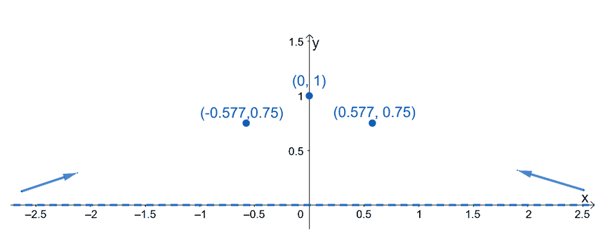
We now have all the information that we need to sketch the curve of $f(x)$. Let’s use all the components of $f(x)$ that we have determined and start graphing $f(x)$.

• Plot the $y$-intercept, $(0, 1)$, and the horizontal asymptote, $y=0$.
• Keep in mind that $(0, 1)$ is also a local maximum of $f(x)$.
• Include the two inflection points of $f(x)$: $\left(-\dfrac{1}{\sqrt{3}},\dfrac{3}{4}\right)$ and $\left(\dfrac{1}{\sqrt{3}},\dfrac{3}{4}\right)$.
• Mark the intervals where $f(x)$ is increasing or decreasing.

Now that we have the crucial points and components plotted on the $xy$-plane, the next step is to use the results from the function’s first and second derivative tests.

• Use the fact that $f(x)$ is increasing at $(-\infty, 0)$ and decreasing at $(0, \infty)$.
• In addition, $f(x)$, is concaving upwards at the intervals $(-\infty, -0.577$ and $(0.577, \infty)$.
• The function is also concaving downwards in between $x=-0.577$ and $x=0.577$ with a maximum point at $(0,1)$.

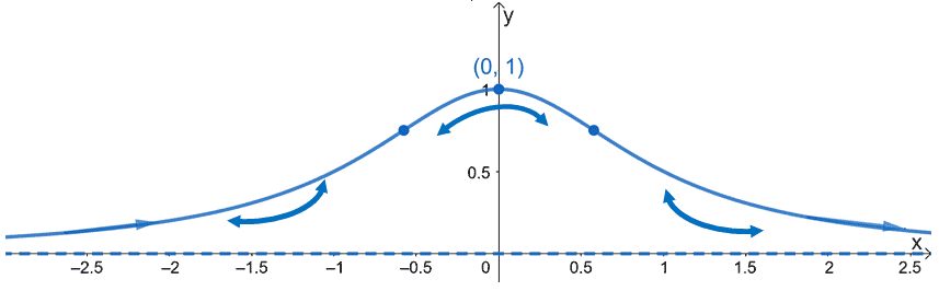
In the current graph that we have, we have confirmed the fact that $f(x)$ is symmetric along the $y$-axis. The graph also confirms the fact that $(0,1)$ is a local maximum. Remove the markers guiding us in sketching $f(x)$’s curve. Hence, we have the simplified graph shown below.

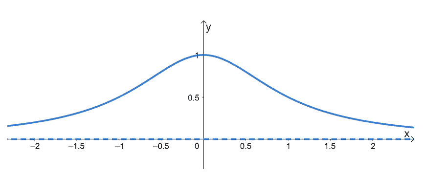
This shows the curve of $f(x) = \dfrac{1}{1 +x^2}$. We’ve just shown you how it’s possible to sketch the curve of a function using its behavior and components.

Summary of curve sketching

Let’s summarize what we know so far and refresh the different properties we’ve used to graph $f(x)$. Make sure to look out for these components when graphing the functions we’ve provided in the next section.

• Determine the intercepts (only when they’re easy to find) and the asymptotes of $f(x)$. Through this, you would also know the domain of $f(x)$.
• When possible, confirm if $f(x)$’s symmetry.
• Differentiate $f(x)$ then equate the expression to $0$. Divide $f(x)$’s domain and find appropriate test values to find $f(x)$’s local extrema.
• Differentiate $f^{\prime}(x)$ and use $f^{\prime\prime}(x)$ to find $f(x)$’s points of inflections. Use this to determine $f(x)$’s concavity.

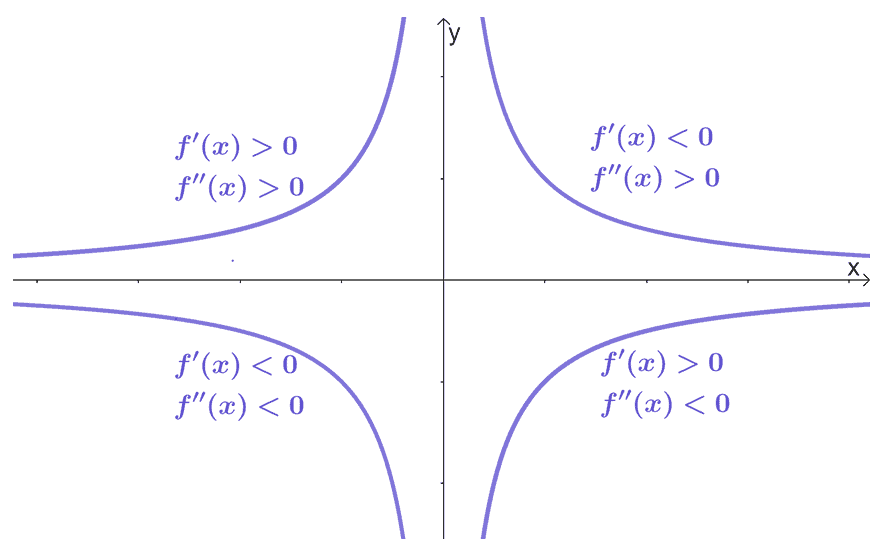
Use this graph as a guide when you’re given the signs of $f^{\prime}(x)$ and $f^{\prime\prime}(x)$ at different intervals. These four different curves are simply there to act as a guide on how a graph may behave at these intervals.

When you’re ready, head over to the questions below to try out the curve sketching steps!

Example 1

Sketch the graph of $f(x) = x^3 − 3 x^2 − 24 x + 32$.

Solution

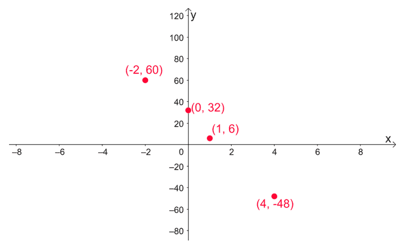
Finding the $x$-intercept for $f(x)$ can be tedious, so we’ll skip this component and instead, move on to finding $f(x)$’s $y$-intercept.

\begin{aligned}f(0) &= 0^3 – 3(0)^2 – 24(0) + 32\\&= 32\\\color{Teal} y_{\text{int}} &\color{Teal} = (0, 32)\end{aligned}

The function, $f(x)$, is a cubic function, so its domain is $\boldsymbol{(-\infty, \infty)}$ and has no asymptotes. Let’s go ahead and see if $f(x)$ is an odd function or not – this will help us in graphing half of $f(x)$’s curve.

\begin{aligned}f(-x)&= (-x)^3  – 3 (-x)^2 – 24(-x) + 32\\&= -x^3 + 3x^2 +24x + 32\\&=-(x^3  -3x^2 -24x – 32)\\&=-f(x)\\&\Rightarrow\color{Orchid}\text{Odd Function}\end{aligned}

This shows that $f(x)$ is an odd function and is symmetric with respect to the origin. Now that we know its fundamental components, let’s proceed with the function’s properties from its first and second derivatives.

We begin by differentiating $f(x)$ using the fundamental derivative rules.

\begin{aligned}f(x)&=x^3- 3 x^2 – 24 x + 32\\ f^{\prime}(x) &= \dfrac{d}{dx}x^3- \dfrac{d}{dx}3 x^2 – \dfrac{d}{dx}24 x + \dfrac{d}{dx}32,\phantom{x}\color{Teal}\text{Sum & Difference Rules} \\&= \dfrac{d}{dx}x^3- {\color{Teal}3\dfrac{d}{dx}x^2 }- {\color{Teal}24\dfrac{d}{dx}x} + {\color{Teal}0},\phantom{x}\color{Teal}\text{Constant & Constant Multiple Rule}\\&= {\color{Teal}3x^2}- 3{\color{Teal}(2x) }- 24{\color{Teal}(1)},\phantom{x}\color{Teal}\text{Power Rule}\\&=3x^2 -6x – 24\end{aligned}

Equate $f^{\prime}(x)$ to zero and solve for the resulting quadratic equation.

\begin{aligned}f^{\prime}(x) &= 0\\3x^2 -6x – 24&= 0\\x^2 -2x -8&= 0\\(x -4)(x + 2)&= 0\\x&=4\\x&= -2\end{aligned}

This means that we can divide the domain of $f(x)$ into smaller intervals using $x= -2$ and $x =4$: $\{(-\infty, -2), (-2, 4), (4, \infty)\}$. Use the test values to see where $f(x)$ is increasing and decreasing.

We’ll also be able to check for local extrema based on $f^{\prime}(x)$’s sign changes.

• Since $f^{\prime}(x)$’s sign changes from $+$ to $-$, $f(x)$ has a local maximum at $(-2, f(-2)) = \boldsymbol{(-2, 60)}$.
• Similarly, since $f^{\prime}(x)$’s sign changes from $-$ to $+$, $f(x)$ has a local minimum at $(4, f(4)) = \boldsymbol{(4, -48)}$.

Let’s move on to the second derivative of $f(x)$ – differentiate $f^{\prime}(x)$ once more.

\begin{aligned}f^{\prime}(x)&=3x^2 -6x – 24\\f^{\prime\prime}(x)&=\dfrac{d}{dx}3x^2 -\dfrac{d}{dx}6x – \dfrac{d}{dx}24,\phantom{x}{\color{Teal}\text{Difference Rule}}\\&={\color{Teal}3\dfrac{d}{dx}x^2} -{\color{Teal}6\dfrac{d}{dx}x} – {\color{Orchid}0},\phantom{x}{\color{Teal}\text{Constant Multiple Rule}}\text{ & }{\color{Orchid}\text{Constant Rule}}\\&= 3{\color{Teal}(2x)} -6{\color{Teal}(1)},\phantom{x}{\color{Teal}\text{Power Rule}}\\&=6x -6\end{aligned}

Find the inflections points of $f(x)$ by equating $f^{\prime\prime}(x)$ to zero.

\begin{aligned}f^{\prime\prime}(x)&= 0\\6x -6 &= 0\\6x &= 6\\x&= 1\\\\f(1) &= (1)^3 -3(1)^2-24(1) + 32\\&= 6\end{aligned}

This means that $f(x)$ has a point of inflection at $\boldsymbol{(1, 6)}$. Check the signs of the function’s second derivative in between the intervals, $(-\infty, 1)$ and $(1, \infty)$, by assigning a test value for each interval. This will tell us whether the function is concaving upward or downward.

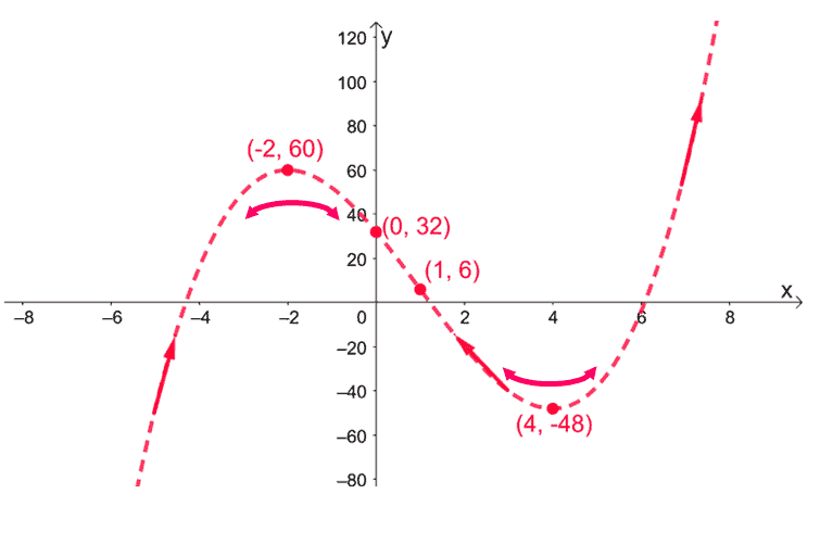
This means that $f(x)$ is concaving downward from the left up to $\boldsymbol{x=1}$ and $f(x)$ is concaving upward from $\boldsymbol{x =1}$ onwards. We now have enough information to sketch the curve of $f(x) = x^3 − 3 x^2 − 24 x + 32$.

Mark the intervals where $x$ is increasing at the intervals $(-\infty, -2)$ and $(4, \infty)$. Mark $(-2, 4)$ as the interval where $f(x)$ is decreasing. Keep in mind that $f(x)$ is also concaving upward at $(-\infty, 1)$ and concaving downward at $(1, \infty)$.

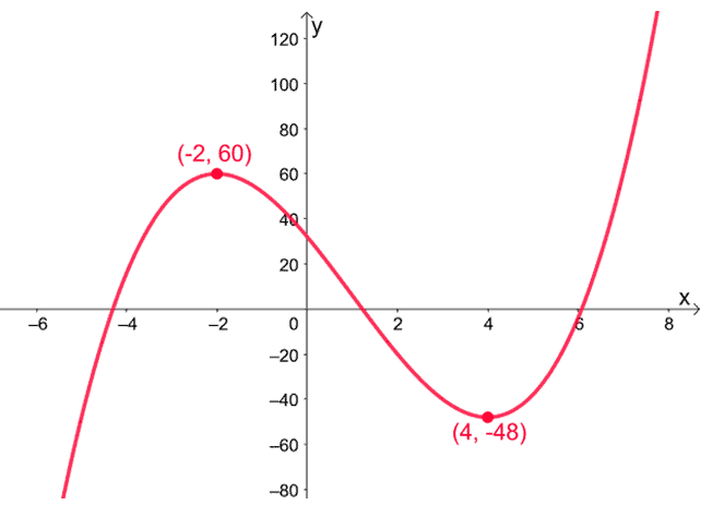
Finalize the graph of $f(x)$ by sketching the full curve using the information that we have – make sure the curve passes through the essential points, is symmetric with respect to the origin, and shares the behavior of $f(x)$ as shown above.

Example 2

Sketch the graph of $g(x) = \dfrac{x^2 + 4}{x -2}$.

Solution

We begin by finding the $x$ and $y$-intercepts of $g(x)$. Equate $g(x)$ to $0$ to find the $x$-intercept of $g(x)$. Find the value of $g(0)$ the $y$-intercept of $g(x)$.

This means that $g(x)$ has no real $x$-intercept and a $\boldsymbol{y}$-intercept at $\boldsymbol{(0, -2)}$. Let’s now determine the vertical asymptote of $g(x)$ by equating its denominator to zero.

\begin{aligned}x -2 &= 0\\x&= 2\end{aligned}

This means that $g(x)$ has a vertical asymptote at $\boldsymbol{x = 2}$. This also tells us that $g(x)$ has a domain of $(-\infty, 2) \cup (2, \infty)$.

Since $g(x)$’s numerator has a higher degree than its denominator, we’re expecting $g(x)$ to have an oblique asymptote. Evaluate $\boldsymbol{\lim_{\infty} \dfrac{g(x)}{x}}$ to finding the oblique asymptote of $g(x)$.

\begin{aligned}g(x) &= \dfrac{x^2 + 4}{x -2}\\&=(x+2) + \dfrac{8}{x – 2}\\\lim_{x \rightarrow \infty}g(x)&= x+2\end{aligned}

This means that $g(x)$ has an oblique asymptote with an equation of $\boldsymbol{x +2}$.

Now that we know the fundamental components of $g(x)$, differentiate $g(x)$ to determine its critical number, extrema, and behavior at different intervals.

\begin{aligned}g(x)&=\dfrac{x^2 + 4}{x -2}\\g^{\prime}(x) &= \dfrac{(x-2)\dfrac{d}{dx}(x^2 +4)- (x^2 +4)\dfrac{d}{dx}(x -2)}{(x -2)^2},\phantom{x}\color{Teal}\text{Quotient Rule}\\ &= \dfrac{(x-2){\color{Teal}\left(\dfrac{d}{dx}x^2 +\dfrac{d}{dx}4\right)}- (x^2 +4){\color{Teal}\left(\dfrac{d}{dx}x -\dfrac{d}{dx}2\right)}}{(x -2)^2},\phantom{x}\color{Teal}\text{Sum & Difference Rules}\\&= \dfrac{(x -2)({\color{Teal}2x} +{\color{Orchid}0}) – (x^2 +4)({\color{Teal}1} -{\color{Orchid}0})}{(x -2)^2},\phantom{x}{\color{Teal}\text{Power Rule}}\text{ & }{\color{Orchid}\text{Constant Rule}}\\&= \dfrac{2x(x -2)- (x^2 +4)}{(x -2)^2}\\&= \dfrac{x^2 – 4x -4}{(x -2)^2}\end{aligned}

Equate $g^{\prime}(x)$ to zero then solve the quadratic equation by applying the quadratic formula.

\begin{aligned}g^{\prime}(x) &= 0\\\dfrac{x^2 – 4x -4}{(x -2)^2}&= 0\\x^2 – 4x – 4 &=0\\x&= \dfrac{-(-4)\pm \sqrt{(-4)^2 – 4(1)(-4)}}{2(1)}\\&= \dfrac{4 \pm 4\sqrt{2}}{2}\\&=2 \pm 2\sqrt{2}\end{aligned}

This means that $g(x)$ has critical numbers at $x = 2 + \sqrt{2}$ and $x = 2- \sqrt{2}$. Let’s use their approximated values to divide the domain of $g(x)$ into smaller intervals.

This table tells us that $g(x)$ has a local maximum and a local minimum.

• Since $g^{\prime}(x)$’s sign has changed from negative to positive at $x=2- 2\sqrt{2}$, $g(x)$ has a local maximum at $(2 -2\sqrt{2}, f(2- 2\sqrt{2})) = \boldsymbol{(2-\sqrt{2}, 4 -4\sqrt{2})}$.
• Since $g^{\prime}(x)$’s sign has changed from positive to negative at $x=2+ 2\sqrt{2}$, $g(x)$ has a local minimum at $(2 +2\sqrt{2}, f(2 + 2\sqrt{2})) = \boldsymbol{(2 + \sqrt{2}, 4 +4\sqrt{2})}$.

After using the first derivative of $g(x)$ to find local extrema, let’s use $g^{\prime\prime}(x)$ to find the inflection points and concavity of $g(x)$. Begin by differentiating $g^{\prime }(x)$ to find $g^{\prime\prime}(x)$.

\begin{aligned}g^{\prime}(x)&= \dfrac{x^2 – 4x – 4}{(x -2)^2}\\g^{\prime\prime}(x)&= \dfrac{(x-2)^2\dfrac{d}{dx}(x^2 -4x -4) – (x^2 -4x -4)\dfrac{d}{dx}(x – 2)^2}{[(x-2)^2]^2},\phantom{x}\color{Teal}{\text{Quotient Rule}}\\&= \dfrac{(x-2)^2\dfrac{d}{dx}(x^2 -4x -4) – (x^2 -4x -4)\dfrac{d}{dx}(x – 2)^2}{(x-2)^4}\end{aligned}

Let’s focus on differentiating the two expressions from the numerator.

Let’s rewrite our current expression for $g^{\prime \prime}(x)$ using the results shown above.

\begin{aligned}g^{\prime\prime}(x)&= \dfrac{(x-2)^2(2x -4) – (x^2 -4x -4)[2(x -2)]}{(x-2)^4}\\&=\dfrac{2(x-2)[(x -2)^2-(x^2 – 4x -4)]}{(x -2)^2}\\&=\dfrac{2(x-2)[x^2 -4x + 4-x^2 + 4x +4)]}{(x -2)^4}\\&= \dfrac{16(x -2)}{(x -2)^4}\\&= \dfrac{16}{(x -2)^3}\end{aligned}

To find the points of inflection, determine the values of $x$ where $g^{\prime \prime}(x)$ is either zero. The second derivative of $g(x)$ can never be zero, so $g(x)$ has no point of inflection.

Test some values using the domain of $g(x)$ and observe the sign of $g^{\prime \prime}(x)$.

This shows that $g(x)$’s curve is concaving upwards at the interval, $(2, \infty)$. Similarly, $g(x)$’s curve is concaving downwards at the interval, $(-\infty, 2)$. Now that we have all the key information about $g(x)$’s curve, let’s begin sketching it.

Begin by plotting the intercepts, asymptotes, and local extrema of $g(x)$.

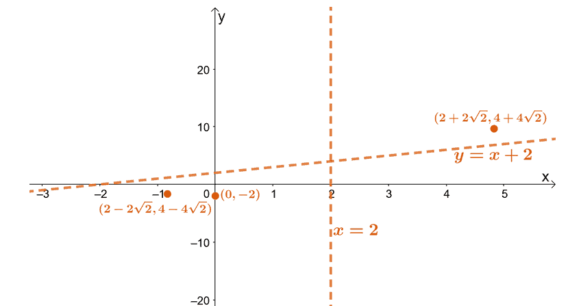
Now, let’s use the intervals where $g(x)$ is increasing and decreasing. Keep in mind where $g(x)$ is concaving upward and downward as well. The asymptotes will help us in sketching the curves since it tells us the regions that $g(x)$’s curve is not allowed to pass through.

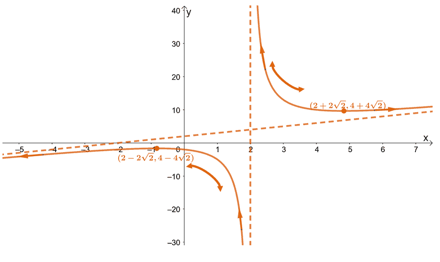
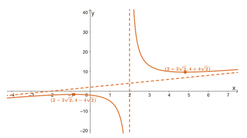
Let’s remove the markers we placed to guide us in sketching the curve of $g(x)$. Below is the final graph of $g(x)$.

Practice Questions

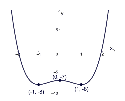
1. Find the following values of the function, $f(x) = x^4 -2x^2 – 7$, then sketch the function’s curve.
a. $y$-intercept
b. Minimum and maximum points (local and global)
c. Points of inflection
d. Intervals where $f(x)$ is increasing and decreasing
e. The concavity of $f(x)$ at different intervals
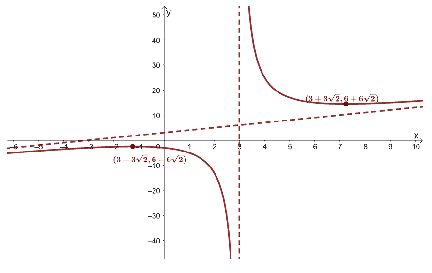
2. Find the following values of the function, $g(x) = \dfrac{x^2 + 9}{x – 3}$, then sketch the function’s curve.
a. $y$-intercept
b. Graph’s asymptotes
c. Minimum and maximum points (local and global)
d. Points of inflection
e. Intervals where $f(x)$ is increasing and decreasing
f. The concavity of $f(x)$ at different intervals

Practice Questions

1.
a. $(0, 7)$
b. Local maximum at $(0, 7)$, global minima at $(-1, 6)$ and $(1, 6)$
c. $\left(-\dfrac{1}{\sqrt{3}}, \dfrac{58}{9}\right)$ and $\left(\dfrac{1}{\sqrt{3}}, \dfrac{58}{9}\right)$
d. Increasing at $(-1, 0)$ and $(1, \infty)$; decreasing at $(-\infty, -1)$ and $(0, 1)$
e. Concaving upwards at $\left(-\infty, -\dfrac{1}{\sqrt{3}}\right)$; concaving downward at $\left(\dfrac{1}{\sqrt{3}},\infty\right)$

2.
a. $(0, -3)$
b. Vertical asymptote: $x = 3$; Oblique asymptote: $y = x +3$
c. Local maximum at $(3- 3\sqrt{2}, 6 – 6\sqrt{2})$, local minimum at $(3+ 3\sqrt{2}, 6 + 6\sqrt{2})$
d. No points of inflection found
e. Increasing at $(-\infty, 3- 3\sqrt{2})$ and $(3 + 3\sqrt{2}, \infty)$; decreasing at $(3 – 3\sqrt{3}, 3)$ and $(3, \infty)$
f. Concaving downward at $\left(-\infty, 3\right)$; concaving upward at $\left(3, \infty\right)$

Images/mathematical drawings are created with GeoGebra.