JUMP TO TOPIC
Covariance depicts the transitions between the two variables, such that a shift in one variable is equal to a transformation in another variable. This is the effect of a function holding its shape when the variables are linearly changed.
Covariance supplies a standard of the stability of correlation among collections of arbitrary variates. The covariance for two random variates X and Y, each with sample size N, is represented by the anticipation value.
Types of Covariance
The covariance equation is operated to specify the focus of the connection between two variables–in other words, whether they grow to move in the exact or opposing directions. This relationship is decided by the symbol(positive or negative) of the covariance value.
A positive covariance among two variables exhibits that these variables overlook to be lower or higher simultaneously. A positive covariance among the variables x and y insinuates that x is more increased than average at the same time that y is more heightened than average, and vice versa. When charted on a two-dimensional chart, the data points will produce to slope upwards.
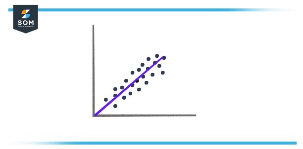
Figure 1 – Positive Covariance
When the prearranged covariance is less than zero, this depicts that the two variables have an inverse connection or negative covariance. In other terms, a value x, which is less than average is paired with a value y which is ampler than average and vice versa.
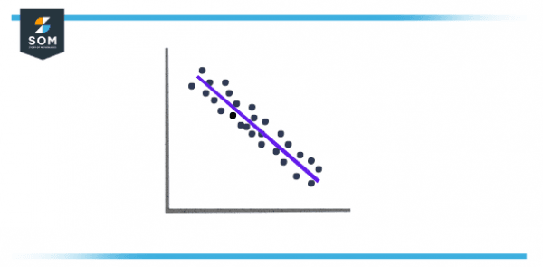
Figure 2 – Negative Covariance
Covariance vs. Variance
Covariance is connected to variance, a statistical measurement for the stretch of points in a data set. Both variance and covariance estimate how data points are allocated around a plotted mean. However, variance counts the distance of data along the x or y in a single direction, and the covariance inspects the directional relationships among two variables.
In the context of economics, covariance is utilized to analyze how additional investments conduct in relation to one another. A positive covariance hints that two assets manage to function simultaneously, while a negative covariance exhibits that they manage to push in opposite paths. Most investors aspire to investments with a negative covariance in decree to diversify their holdings.
Covariance vs. Correlation
Covariance is also different from correlation, another statistical metric frequently utilized to count the relationship between two variables. While covariance estimates the approach of a relationship between two variables, correlation estimates the stability of that relationship. This is usually depicted through a correlation coefficient, which can vary from -1 to +1.
While the covariance does calculate the directional relationship between two purchases, it does not show the power of the relationship between the two purchases; the coefficient of correlation is a better suitable indicator of this power.
A correlation is assessed to be powerful if the coefficient of correlation is close to +1 which is a positive correlation or -1 which is a negative correlation. A coefficient which is near zero implies that there is only a weak collaboration between the two variables.
Similarities Between Covariance and Correlation
Correlation and Covariance both gauge the unbent relationships between two variables solely. When the coefficient of correlation is zero, the covariance is also zero. Both correlation and covariance estimates are also unchanged by the transformation in the area.
Nevertheless, when it arrives to creating a preference between covariance and correlation to measure the connection between variables, correlation is chosen over covariance because it does not obtain involved by the transformation in scale.
Calculating Covariance
For two variables x and y, the covariance is reckoned by accepting the contrast between each x and y variable and their separate standards. These distinctions are then multiplied concurrently and averaged across all of the data points. In the mathematical inscription, this is represented as:
\[ Cov(x, y) = \sum_{K=0}^i \dfrac{(x_i – \overline{x}) \times (y_i – \overline{y} )}{n-1} \]
The covariance value can vary from -∞ to +∞, with a negative value denoting a negative relationship and a positive value showing a positive relationship. The more renowned this number, the more reliant the relationship. Positive covariance suggests a direct connection and is conveyed by a positive number.
A negative number, on the other hand, characterizes negative covariance, which tells an inverse relationship between the two variables. Covariance is significant for describing the type of relationship, but it’s horrible for decoding the magnitude.
Covariance Matrix
A square matrix supplies the covariance between each duo of segments(or elements) of a provided spontaneous vector is named a covariance matrix. The covariance matrix is symmetric and is also positive and semi-definite. The principal sloping or main sloping (sometimes a primary diagonal) of this matrix organizes variances. That indicates the covariance of each part with itself. A covariance matrix is also understood as the auto-covariance matrix, variance matrix also dispersion matrix, or variance-covariance matrix.
Application Of Covariance
Covariance is being utilized in affecting systems with numerous correlated variables is accomplished by utilizing Cholesky decomposition. A covariance matrix enables determining the Cholesky decomposition because it is positive and semi-definite. The matrix is deteriorated by the outcome of the lower matrix and its transpose.
An Example of Analyzing Data With Covariance
Imagine an analyst in a firm who has a data set of 5 years that indicates yearly gross domestic product (GDP) gain in percentages (x) and a company’s new product line expansion in percentages (y). The data set may glance like this:
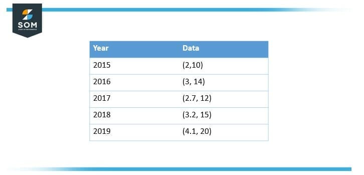
Figure 3 – Yearly Report of GDP
What can analysts express regarding the elaboration of the company’s recent product line?
Solution
The par x value equals 3, and the moderate y value equals 14.2. That can be calculated as follows,
\[ \overline{x} = \dfrac{2+ 3+ 2.7+ 3.2+ 4.1}{5} \]
\[ \overline{x} = 3 \]
And besides $\overline{y}$
\[ \overline{y} = \dfrac{10+ 14+ 12 +15 + 20}{5} \]
\[ \overline{y} = 14.2 \]
To estimate the covariance, the aggregate of the products of the $x_i$ values subtracts the average x value $\overline{x}$, multiplied by the $y_i$ values subtracted from the average y values $ \overline{y}$ can be divided by (n-1), as follows:
Enclosing computed a positive covariance here, the analyst can state that the development of the company’s new product line has a positive association with yearly GDP development.
All images/mathematical drawings were created with GeoGebra.