Linear Equation|Definition & Meaning

An equation refers to a mathematical argument where the algebraic statement is separated by an equivalent sign (=). 

The first-degree equations are known as linear equations. linear equations represent a straight line. When variables are replaced with unknown variables in linear equations, the results produce values that make the equation valid. There is just one answer when there is just one variable.

For instance, y = -5 is the unique answer to the equation y + 5 = 0. However, in the scenario of the linear equation involving two or more variables, the results are determined in the form of the Cartesian coordinates of a particular point in Euclidean space.

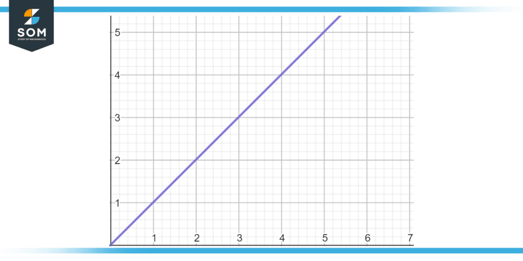
Figure 1: Graphical Illustration of Linear Equation

Different Forms of a Linear Equation

According to the variables and constants included in a linear equation, there are four ways to express a linear equation. These four forms of a linear equation are described below.

General Form

In the general form of the linear equation, the equation is expressed in the following form y.

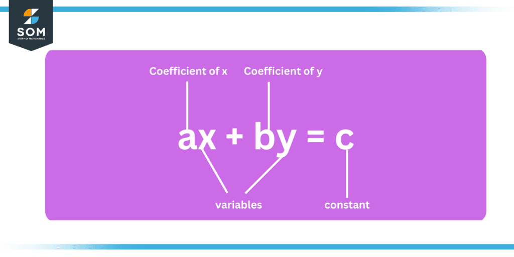
Figure 2: General form of linear equation

For instance, 3x + 2y = 8 is a linear equation in its general form.

Standard Form

This form of a linear equation is expressed as:

ax + b = c

where x is known as the variable whereas a, b, and c are known as constants. For instance, 5x + 3 = 12 is the linear equation in its standard form.

Slope-Intercept Form

In the slope-intercept form of the linear equation, the equation is expressed in the following form:

y = mx + b

wherein m is the line’s slope, x is known as a variable, and b is known as a y-intercept. For instance, y = 5x + 3 is the linear equation in its slope-intercept form.

Point-Slope Form

In the point-slope form of the linear equation, the equation is expressed in the following form:

y – y1 = m (x – x1)

wherein m is known as the line’s slope, (x1, y1) denotes a point on the line, and x and y are the variables. For instance, y – 4 = 3(x – 2) is a linear equation in its point-slope form.

These varying forms of a linear equation can be transformed into one another using algebraic methods and are helpful in various contexts.  For instance, by reorganizing the components and solving for y, we can change a linear equation in its standard form to a linear equation in its slope-intercept form.

Likewise, we can change a linear equation from slope-intercept form to point-slope form by locating a position on the line and inserting it into the equation.

How To Solve a Linear Equation

We can solve a linear by employing three methods. Each of these three methods is discussed below.

Addition Method of Solving a Linear Equation

To separate the variable in the linear equation and determine its value, this method requires adding an identical number to both sides of the equation. For instance, to solve the following equation,

5x + 2 = 12

We can subtract 2 from both sides of the equation to get:

5x = 10

After that, we can multiply both sides with 1/5 to obtain x = 2.

Multiplication Method of Solving a Linear Equation

This technique requires multiplying the same number on both sides of the equation, to separate the variable in the linear equation and determine its value. For instance, in the case of solving the following equation

5x + 2 = 12

We will multiply both sides of the equation by 1/5 to obtain the following:

x + 2/5 = 12/5

Now, we may subtract 2/5 from both sides of the equation to achieve the following:

x = 10/5

Substitution Method of Solving a Linear Equation

This approach entails changing one of the equation’s variables for an expression that also includes the other variable.

Let us say we have two equations:

a + b = 5

a – b = 3

Now, we can get the value of x from the 1^st equation and then use it as a substitution in the 2^nd equation. As a result, we obtain:

b = 5 – a

a – b = 3

By calculating for ‘a’ in the 2^nd equation and using the result as a replacement in the 1^st equation, we arrive at the following solutions.

a – (5 – a) = 3

This gives us the following value of ‘a.’

a = 4

Now putting the value of ‘a’ in the first equation gives us the following value of b.

b = 1

These approaches for linear equations include manipulating the equations and isolating the variables by utilizing algebraic methods. The equation in hand and the provided information will determine the right approach to employ. These techniques allow us to solve linear equations and employ the results to represent scenarios in the actual world.

How To Plot Linear Equations?

The slope or gradient as well as the y-intercept of a line must be determined in order to plot a linear equation. The y-intercept, or a point at which the line intersects the y-axis, is what determines the slope. Whereas slope is ascertained by the coefficient of the equation’s value of x.

The y-intercept can be plotted on the reference plane after the slope and y-intercept have been calculated. Next, we locate a second point on the line by using the slope.

For instance, if the slope of the line is 3, we can identify a second point on the line by adding 3 in the x-coordinate of the y-intercept. Given that the line has no uphill or downhill slope in this instance, the y-coordinate of the second point will be similar to that of the y-intercept.

When we have located 2 points on a line representing a linear equation, we can plot the equation by connecting both with a straight line. The line emerging as an outcome represents the linear equation’s answer.

For example, take into account the following linear equation:

y = 3x + 2.

We must first identify the gradient and y-intercept in order to graph this equation. Given that the line intersects the y-axis at y = 2, the slope or gradient of the line is 3, and the y-intercept of the line is (0, 2).

The y-intercept is then plotted on the coordinate plane. Next, we locate a 2n point on the line by using the slope. This can be done by adding 3 to the x-coordinate of the y-intercept because the slope is 3. Given that the line has no uphill or downhill slope in this instance, the y-coordinate of the second point coincides with the y-intercept. As a result, the second line segment is (3, 2).

The equation is then graphed by drawing a straight line connecting the two spots. The answer to the linear equation y = 3x + 2 is the resultant line.

Examples of Linear Equations

Example 1

Solve the following linear equation:

4x + 6 = 14

Solution

Given equation:

4x + 6 = 14

First of all, we have to isolate the variable:

4x = 14 – 6

Performing the subtraction on the RHS:

4x = 8

Dividing both sides by 4:

x = 2

Example 2

Solve the following linear equation:

5x + 6 = 2x + 18

Solution

5x + 6 = 2x + 18

First of all, we have to isolate the variable:

5x – 2x = 18 – 6

Solving further:

3x = 12

x = 4

Example 3

Plot the following linear equation:

3y = 2x + 3

Solution

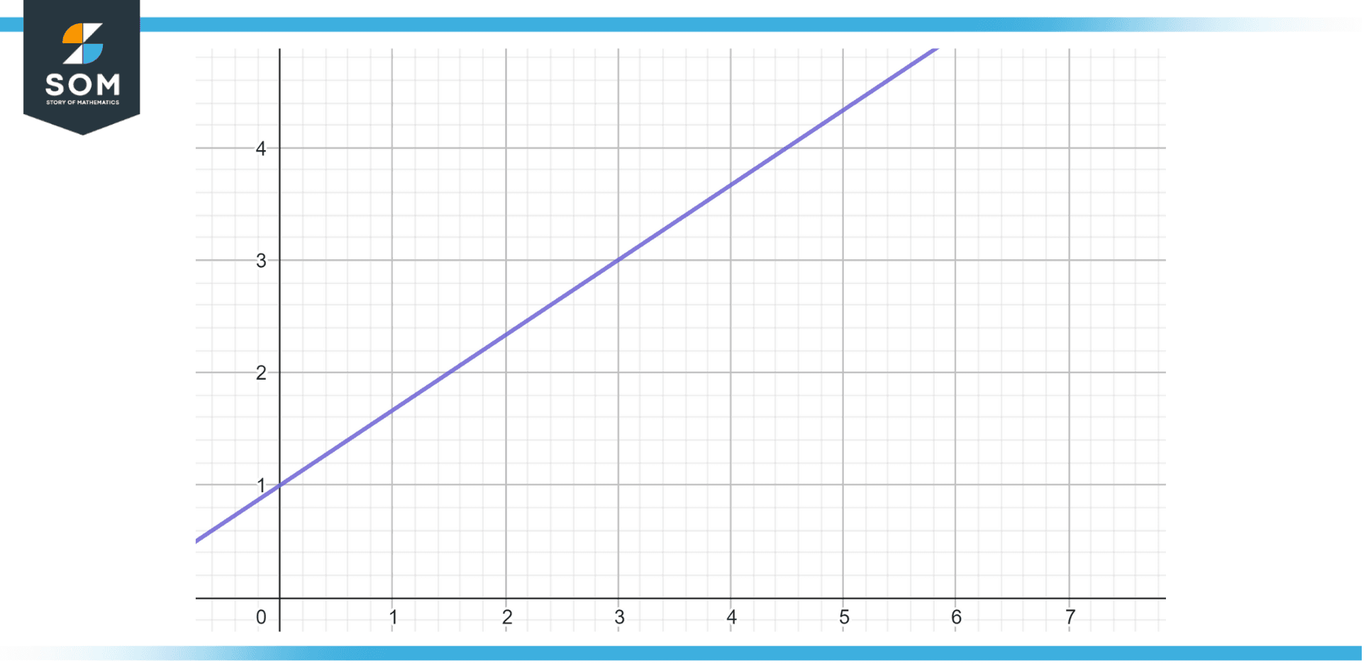
Figure 3: Solution of Example 3

All images/mathematical drawings were created with GeoGebra.

Line Symmetry Definition < Glossary Index > Logarithmic Scale Definition