JUMP TO TOPIC
Lagrange Multiplier Calculator + Online Solver With Free Steps
The Lagrange Multiplier Calculator finds the maxima and minima of a function of n variables subject to one or more equality constraints. If a maximum or minimum does not exist for an equality constraint, the calculator states so in the results.
The constraints may involve inequality constraints, as long as they are not strict. However, equality constraints are easier to visualize and interpret. Valid constraints are generally of the form:
\[ x_1^2+x_2^2 \geq a \]
\[ 3x_1 + x_3 \leq b \]
x2 – x3 = c
Where a, b, c are some constants. Since the main purpose of Lagrange multipliers is to help optimize multivariate functions, the calculator supports multivariate functions and also supports entering multiple constraints.

What Is the Lagrange Multiplier Calculator?
The Lagrange Multiplier Calculator is an online tool that uses the Lagrange multiplier method to identify the extrema points and then calculates the maxima and minima values of a multivariate function, subject to one or more equality constraints.
The calculator interface consists of a drop-down options menu labeled “Max or Min” with three options: “Maximum,” “Minimum,” and “Both.” Picking “Both” calculates for both the maxima and minima, while the others calculate only for minimum or maximum (slightly faster).
Additionally, there are two input text boxes labeled:
- “Function”: The objective function to maximize or minimize goes into this text box.
- “Constraint”: The single or multiple constraints to apply to the objective function go here.
For multiple constraints, separate each with a comma as in “x^2+y^2=1, 3xy=15” without the quotes.
How To Use the Lagrange Multiplier Calculator?
You can use the Lagrange Multiplier Calculator by entering the function, the constraints, and whether to look for both maxima and minima or just any one of them. As an example, let us suppose we want to enter the function:
f(x, y) = 500x + 800y, subject to constraints 5x+7y $\leq$ 100, x+3y $\leq$ 30
Now we can begin to use the calculator.
Step 1
Click on the drop-down menu to select which type of extremum you want to find.
Step 2
Enter the objective function f(x, y) into the text box labeled “Function.” In our example, we would type “500x+800y” without the quotes.
Step 3
Enter the constraints into the text box labeled “Constraint.” For our case, we would type “5x+7y<=100, x+3y<=30” without the quotes.
Step 4
Press the Submit button to calculate the result.
Results
The results for our example show a global maximum at:
\[ \text{max} \left \{ 500x+800y \, | \, 5x+7y \leq 100 \wedge x+3y \leq 30 \right \} = 10625 \,\, \text{at} \,\, \left( x, \, y \right) = \left( \frac{45}{4}, \,\frac{25}{4} \right) \]
And no global minima, along with a 3D graph depicting the feasible region and its contour plot.
3D And Contour Plots
If the objective function is a function of two variables, the calculator will show two graphs in the results. The first is a 3D graph of the function value along the z-axis with the variables along the others. The second is a contour plot of the 3D graph with the variables along the x and y-axes.
How Does the Lagrange Multiplier Calculator Work?
The Lagrange Multiplier Calculator works by solving one of the following equations for single and multiple constraints, respectively:
\[ \nabla_{x_1, \, \ldots, \, x_n, \, \lambda}\, \mathcal{L}(x_1, \, \ldots, \, x_n, \, \lambda) = 0 \]
\[ \nabla_{x_1, \, \ldots, \, x_n, \, \lambda_1, \, \ldots, \, \lambda_n} \, \mathcal{L}(x_1, \, \ldots, \, x_n, \, \lambda_1, \, \ldots, \, \lambda_n) = 0 \]
Usage of Lagrange Multipliers
The Lagrange multiplier method is essentially a constrained optimization strategy. Constrained optimization refers to minimizing or maximizing a certain objective function f(x1, x2, … , xn) given k equality constraints g = (g1, g2, … , gk).
Intuition
The general idea is to find a point on the function where the derivative in all relevant directions (e.g., for three variables, three directional derivatives) is zero. Visually, this is the point or set of points $\mathbf{X^*} = (\mathbf{x_1^*}, \, \mathbf{x_2^*}, \, \ldots, \, \mathbf{x_n^*})$ such that the gradient $\nabla$ of the constraint curve on each point $\mathbf{x_i^*} = (x_1^*, \, x_2^*, \, \ldots, \, x_n^*)$ is along the gradient of the function.
As such, since the direction of gradients is the same, the only difference is in the magnitude. This is represented by the scalar Lagrange multiplier $\lambda$ in the following equation:
\[ \nabla_{x_1, \, \ldots, \, x_n} \, f(x_1, \, \ldots, \, x_n) = \lambda \nabla_{x_1, \, \ldots, \, x_n} \, g(x_1, \, \ldots, \, x_n) \]
This equation forms the basis of a derivation that gets the Lagrangians that the calculator uses.
Note that the Lagrange multiplier approach only identifies the candidates for maxima and minima. It does not show whether a candidate is a maximum or a minimum. Usually, we must analyze the function at these candidate points to determine this, but the calculator does it automatically.
Solved Examples
Example 1
Maximize the function f(x, y) = xy+1 subject to the constraint $x^2+y^2 = 1$.
Solution
In order to use Lagrange multipliers, we first identify that $g(x, \, y) = x^2+y^2-1$. If we consider the function value along the z-axis and set it to zero, then this represents a unit circle on the 3D plane at z=0.
We want to solve the equation for x, y and $\lambda$:
\[ \nabla_{x, \, y, \, \lambda} \left( f(x, \, y)-\lambda g(x, \, y) \right) = 0 \]
Getting the Gradients
First, we find the gradients of f and g w.r.t x, y and $\lambda$. Knowing that:
\[ \frac{\partial}{\partial \lambda} \, f(x, \, y) = 0 \,\, \text{and} \,\, \frac{\partial}{\partial \lambda} \, \lambda g(x, \, y) = g(x, \, y) \]
\[ \nabla_{x, \, y, \, \lambda} \, f(x, \, y) = \left \langle \frac{\partial}{\partial x} \left( xy+1 \right), \, \frac{\partial}{\partial y} \left( xy+1 \right), \, \frac{\partial}{\partial \lambda} \left( xy+1 \right) \right \rangle\]
\[ \Rightarrow \nabla_{x, \, y} \, f(x, \, y) = \left \langle \, y, \, x, \, 0 \, \right \rangle\]
\[ \nabla_{x, \, y} \, \lambda g(x, \, y) = \left \langle \frac{\partial}{\partial x} \, \lambda \left( x^2+y^2-1 \right), \, \frac{\partial}{\partial y} \, \lambda \left( x^2+y^2-1 \right), \, \frac{\partial}{\partial \lambda} \, \lambda \left( x^2+y^2-1 \right) \right \rangle \]
\[ \Rightarrow \nabla_{x, \, y} \, g(x, \, y) = \left \langle \, 2x, \, 2y, \, x^2+y^2-1 \, \right \rangle \]
Solving the Equations
Putting the gradient components into the original equation gets us the system of three equations with three unknowns:
\[ y-\lambda 2x = 0 \tag*{$(1)$} \]
\[ x-\lambda 2y = 0 \tag*{$(2)$} \]
\[ x^2+y^2-1 = 0 \tag*{$(3)$} \]
Solving first for $\lambda$, put equation (1) into (2):
\[ x = \lambda 2(\lambda 2x) = 4 \lambda^2 x \]
x=0 is a possible solution. However, it implies that y=0 as well, and we know that this does not satisfy our constraint as $0 + 0 – 1 \neq 0$. Instead, rearranging and solving for $\lambda$:
\[ \lambda^2 = \frac{1}{4} \, \Rightarrow \, \lambda = \sqrt{\frac{1}{4}} = \pm \frac{1}{2} \]
Substituting $\lambda = +- \frac{1}{2}$ into equation (2) gives:
\[ x = \pm \frac{1}{2} (2y) \, \Rightarrow \, x = \pm y \, \Rightarrow \, y = \pm x \]
Putting x = y in equation (3):
\[ y^2+y^2-1=0 \, \Rightarrow \, 2y^2 = 1 \, \Rightarrow \, y = \pm \sqrt{\frac{1}{2}} \]
Which means that $x = \pm \sqrt{\frac{1}{2}}$. Now put $x=-y$ into equation $(3)$:
\[ (-y)^2+y^2-1=0 \, \Rightarrow y = \pm \sqrt{\frac{1}{2}} \]
Which means that, again, $x = \mp \sqrt{\frac{1}{2}}$. Now we have four possible solutions (extrema points) for x and y at $\lambda = \frac{1}{2}$:
\[ (x, y) = \left \{\left( \sqrt{\frac{1}{2}}, \sqrt{\frac{1}{2}} \right), \, \left( \sqrt{\frac{1}{2}}, -\sqrt{\frac{1}{2}} \right), \, \left( -\sqrt{\frac{1}{2}}, \sqrt{\frac{1}{2}} \right), \, \left( -\sqrt{\frac{1}{2}}, \, -\sqrt{\frac{1}{2}} \right) \right\} \]
Classifying the Extrema
Now to find which extrema are maxima and which are minima, we evaluate the function’s values at these points:
\[ f \left(x=\sqrt{\frac{1}{2}}, \, y=\sqrt{\frac{1}{2}} \right) = \sqrt{\frac{1}{2}} \left(\sqrt{\frac{1}{2}}\right) + 1 = \frac{3}{2} = 1.5 \]
\[ f \left(x=\sqrt{\frac{1}{2}}, \, y=-\sqrt{\frac{1}{2}} \right) = \sqrt{\frac{1}{2}} \left(-\sqrt{\frac{1}{2}}\right) + 1 = 0.5 \]
\[ f \left(x=-\sqrt{\frac{1}{2}}, \, y=\sqrt{\frac{1}{2}} \right) = -\sqrt{\frac{1}{2}} \left(\sqrt{\frac{1}{2}}\right) + 1 = 0.5 \]
\[ f \left(x=-\sqrt{\frac{1}{2}}, \, y=-\sqrt{\frac{1}{2}} \right) = -\sqrt{\frac{1}{2}} \left(-\sqrt{\frac{1}{2}}\right) + 1 = 1.5\]
Based on this, it appears that the maxima are at:
\[ \left( \sqrt{\frac{1}{2}}, \, \sqrt{\frac{1}{2}} \right), \, \left( -\sqrt{\frac{1}{2}}, \, -\sqrt{\frac{1}{2}} \right) \]
And the minima are at:
\[ \left( \sqrt{\frac{1}{2}}, \, -\sqrt{\frac{1}{2}} \right), \, \left( -\sqrt{\frac{1}{2}}, \, \sqrt{\frac{1}{2}} \right) \]
We verify our results using the figures below:
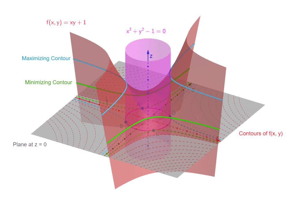
Figure 1
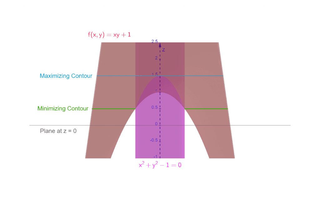
Figure 2
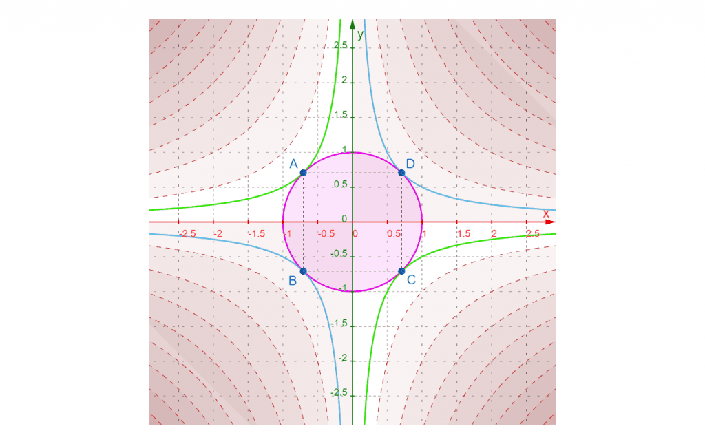
Figure 3
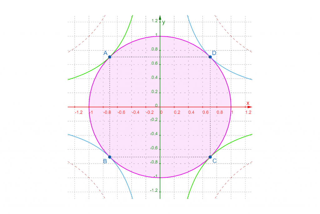
Figure 4
You can see (particularly from the contours in Figures 3 and 4) that our results are correct! The calculator will also plot such graphs provided only two variables are involved (excluding the Lagrange multiplier $\lambda$).
All Images/Mathematical drawings are created using GeoGebra.