JUMP TO TOPIC
Linearization Calculator + Online Solver With Free Steps
The Linearization Calculator is used to compute the linearization of a function at a given point. The point a lies on the curve of the function f(x). The calculator provides a tangent line at the given point a on the input curve. Linearization is an essential tool in approximating the curved function into a linear function at a given point on the curve.It computes the Linearization function, which is a tangent line drawn at the point a on the function f(x).The Linearization function L(x) of a function f(x) at a given point a is obtained by using the formula as follows:L(x) = f(a) + f´(a) (x – a)
Here, f(a) represents the value of the function f(x) after substituting the value of a in it.The function f´(x) is obtained by taking the first derivative of the function f(x). The value of f´(a) comes by putting the value of a in the derivative of the function f’(x).The point a lies on the function f(x). The function f(x) is a non-linear function. It is a function with a degree greater than 1.The calculator gives a slope-intercept form of the linearization function L(x) and also provides a plot for the function f(x) and L(x) in the x-y plane.
What Is a Linearization Calculator?
The Linearization Calculator is an online tool that is used to calculate the equation of a linearization function L(x) of a single-variable non-linear function f(x) at a point a on the function f(x).The calculator also plots the graph of the non-linear function f(x) and the linearization function L(x) in a 2-D plane. The linearization function is a tangent line drawn at the point a on the curve f(x).The Linearization formula used by the calculator is the Taylor series expansion of first order.The Linearization Calculator has a wide range of usage when dealing with non-linear functions. It is used to approximate the non-linear functions into linear functions that change the shape of the graph.How To Use the Linearization Calculator
The user can follow the steps given below to use the Linearization Calculator.Step 1
The user must first enter the function f(x) for which the linearization approximation is required. The function f(x) should be a non-linear function with a degree greater than one.It is entered in the block titled, “linear approximation of” in the calculator’s input window.The calculator takes the function as a one-variable function of x by default. The user should not use another variable in the non-linear function.The calculator uses the function as given below by default for which the linearization approximation is calculated:\[ f(x) = x^4 + 6 x^{2} \]It is a non-linear function with a degree of 4.Step 2
The user must now enter the point at which the linearization approximation is needed. This point lies on the curve or the non-linear function f(x). The point is named as a by the calculator.It is entered in the block labeled ”when a=” in the calculator’s input window.This is the point at which the tangent line is drawn on the input curve which gives the linear approximation.The calculator sets the value of a by default as:a = – 1
It lies on the function $f(x) = x^4 + 6 x^{2}$. The calculator computes the linearization equation of the function f(x) at the point a.Step 3
The user must now enter the “Submit” button for the calculator to compute the output. If a two-variable function f(x,y) is entered in the block “linear approximation of”, the calculator gives the signal “Not a valid input; please try again”.If the value of a entered by the user is incorrect or not an integer, the calculator again gives the signal that the input is not valid.Output
The calculator processes the input data and computes the output in the three windows given below.Input Interpretation
The calculator interprets the input and displays it in this window. For the default example, it displays the input as follows:\[ tangent \ line \ \ to \ y = x^4 + 6 x^{2} \ \ at \ a = – \ 1 \]It shows that the calculator will compute the equation for the tangent line on the non-linear function at the point a on the curve.The user can verify the entered input from the input interpretation window whether the calculator has taken the input according to the user’s requirements.Result
The Result’s window shows the linear approximation of the function f(x) at the point a on the curve. The calculator computes an equation which is the “slope-intercept form” of the linearization function L(x).This equation is obtained by using the Linearization formula for the linearization function L(x), that is:L(x) = f(a) + f´(a) (x – a)
The calculator also provides all the mathematical steps required for the particular problem by clicking on “Need a step-by-step solution for this problem?” For the default example, the mathematical steps are given as follows.For the default example, the function f(x) and the point a is given as:\[ f(x) = x^4 + 6 x^{2} \]a = – 1
The value for f(a) is obtained by putting the value of a in the non-linear function f(x) as follows:f(a) = f(- \ 1) = $(- \ 1)^{4}$ + 6 $(- 1)^{2}$ = 1 + 6
f(a) = 7
For f´(a), the first derivative of the function f(x) is given as follows:\[ f´(x) = \frac{ d ( x^4 + 6 x^{2} ) }{ dx } = 4 x^{3} + 6 ( 2x) \]\[ f´(x) = 4 x^{3} + 12x \]Th value of a = -1 is placed into the function f´(x) to obtain f´(a) as follows:f´(- 1) = 4 $(- 1)^{3}$ + 12(- 1) = 4(- 1) – 12 = – 4 – 12
f´(- 1) = – 16
Putting the value of f(a), f´(a), and a in the equation of L(x) gives the linearization approximation at the point a on the curve.L(x) = f(a) + f’(a) (x – a)
L(x) = 7 + (- 16) ( x – (- 1) ) = 7 – 16x – 16
L(x) = – 16x – 9
The calculator shows the Result for the linear approximation as follows:y = – 16x – 9
Plot
The Linearization Calculator also provides a graph plot for the linearization approximation of f(x) at the point a in a x-y plane.The plot shows the non-linear curve of the function f(x). It also displays the linear approximation at the point a, which is a tangent line drawn at the point a on the curve.Solved Examples
Here are some of the examples solved through the Linearization Calculator.Example 1
For the non-linear function:\[ f(x) = 2 x^{3} \]Calculate the linear approximation of the function f(x) at the point a on the curve given as:a = 1
Also plot the curve f(x) and the linearization function L(x) in a 2-D plane.Solution
The user must first enter the non-linear function f(x) and the point a in the input window of the Linearization Calculator.After pressing “Submit”, the calculator opens the output window which shows the three windows as given below.The Input Interpretation window shows the entered input by the user. For this example, it displays the input as follows:tangent line to y = 2 $x^{3}$ at a = 1
The Result’s window displays the equation for the linear approximation L(x) of the function at the given point as follows:y = 6x – 4
The calculator also displays the plot for the function f(x) and the linearization equation L(x) as shown in figure 1.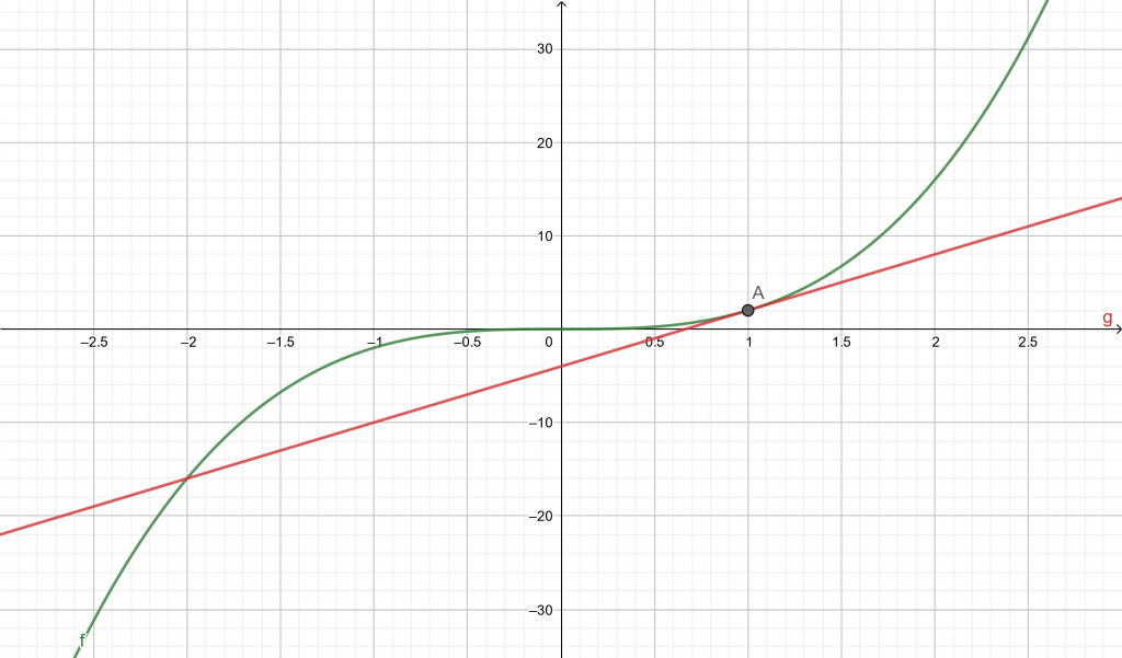
Figure 1
Example 2
Compute the linearization equation for the function:\[ f(x) = 4x^{2} + 1 \]At the point:a = 2
Also plot the graph for f(x) and the linearization equation L(x).Solution
The function f(x) and the point a is entered in the input window of the Linearization Calculator. The user submits the input data and the calculator first shows the Input Interpretation as follows:tangent line to y = 4 $x^{2}$ + 1 at a = 2
The Result’s window displays the linearization equation as follows:y = 16x – 15
The Plot for the non-linear function f(x) and the linearization equation L(x), which is a tangent line drawn at the point a on the curve is shown in figure 2 given below.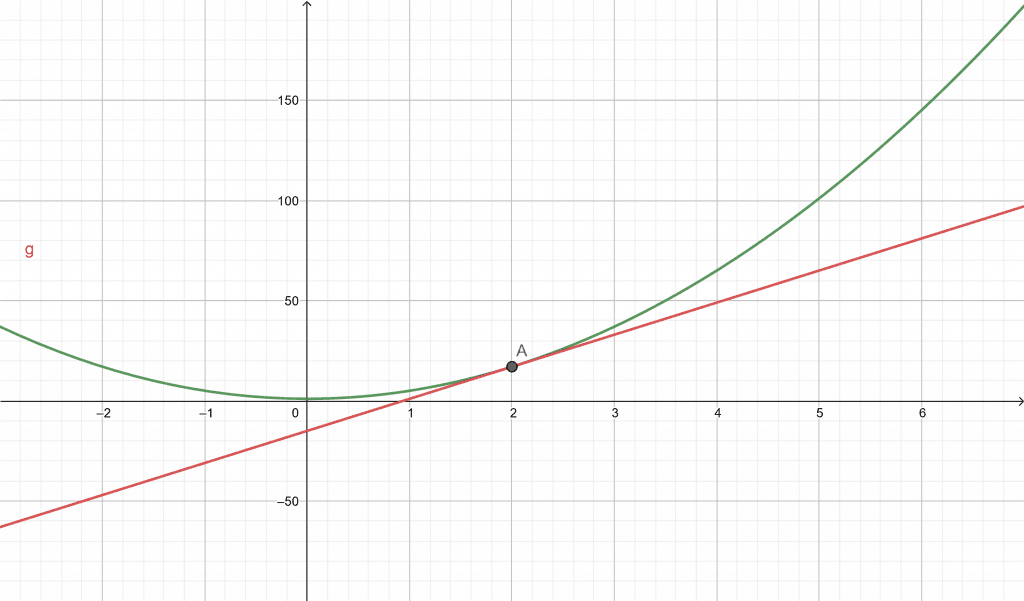
Figure 2