JUMP TO TOPIC
Parametric Equation Calculator + Online Solver With Free Steps
A Parametric Equation Calculator is used to calculate the results of parametric equations corresponding to a Parameter. This calculator in particular works by solving a pair of parametric equations which correspond to a singular Parameter by putting in different values for the parameter and computing results for main variables.
The Calculator is very easy to use and it works by entering your data in the input boxes of the calculator. It also is designed to showcase how the Parametric Equations form a geometry as a result of the 2 dimensions.

What Is a Parametric Equation Calculator?
A Parametric Equation Calculator is an online calculator that can solve your parametric equation problems inside your browser without any pre-requisites.
This Calculator is a standard calculator with not a lot of complex processing going on. This calculator can solve the set of 2-dimensional parametric equations for multiple different inputs of the common independent variable also referred to as the Parameter.
The value of the Parameter is chosen arbitrarily for solving these equations, as it records the response which is generated by the output variables. This response is what these variables describe, and the shapes they draw.
How to Use the Parametric Equation Calculator?
To use the Parametric Equation Calculator, you must have two parametric equations set up, one for x, and the other one for y. These equations must have the same Parameter in them, commonly used as $t$ for time.
Finally, you can get your results at the push of a button. Now, to get the best results from this calculator, you can follow the step-by-step guide given below:
Step 1
First, set up the input parametric equations properly, which means keeping the parameter the same.
Step 2
Now, you can enter the equations in their respective input boxes which are labeled as: solve y = and x =.
Step 3
Once you have entered the inputs into the corresponding input boxes, you can follow that up by pressing the “Submit” button. This will produce your desired results.
Step 4
Finally, if you intend to reuse this calculator, then you can simply enter new problems following every step given above to get as many solutions as you like.
It may be important to note that this calculator is equipped with only a 2-Dimension parametric equation solver, which means it can solve 3-Dimensional or higher problems. The number of parametric equations corresponding to the output variables is associated with the number of dimensions the Parameterization deals with.
How Does the Parametric Equation Calculator Work?
A Parametric Equation Calculator works by solving the parametric equation’s algebra using arbitrary values for the parameter serving as the independent variable in it all. This way we can build a small table-type information set that can be further used to draw out the curves created by said parametric equations.
Parametric Equations
This is a group of equations that are represented by a common Independent Variable which allows them to correspond with one another. This special independent variable is more commonly referred to as the Parameter of these Parametric Equations.
Parametric Equations are normally used for showcasing geometric data, therefore for drawing surfaces, and curves of a Geometry that would be defined by those equations.
This process is usually referred to as Parameterization, whilst the parametric equations may be known as Parametric Representations of said geometries. Parametric equations are usually of the form:
x = f1(t)
y = f2(t)
Where x and y are the parametric variables, whilst t is the Parameter, which in this case is representing “time” as the independent variable.
Example of Parametric Equations
As we discussed above, Parametric Equations are mainly used for describing and drawing geometric shapes. These may include curves and surfaces and even basic geometric shapes such as the Circle. The circle is one of the baseline shapes to exist in geometry and is described parametrically as follows:
x = cos t
y = sin t
The combination of these two variables tends to describe the behavior of a point in the cartesian plane. This point lies on the circumference of the circle, the coordinates of this point can be seen as follows, expressed in the form of a vector:
(x, y) = (cos t, sin t)
Parametric Equations in Geometry
Now, Parametric Equations are also capable of expressing algebraic orientations of higher dimensions along with descriptions of manifolds whereas another important fact to notice regarding these Parametric Equations is that the number of these equations corresponds to the number of dimensions involved. Thus, for 2 dimensions, the number of equations would be 2, and vice versa.
Similar Parametric Representations may also be observed in the field of kinematics, where a parameter $t$ is used which corresponds to time as an Independent Variable. Thus, changes in states of objects corresponding to their trajected paths are represented against Time.
An important fact to observe would be those Parametric Equations and the process of describing these events in terms of a Parameter is not unique. Thus, there may be many different representations of the same shape or trajectory in Parameterization.
Parametric Equations in Kinematics
Kinematics is a branch of physics dealing with objects in motion or at rest, and Parametric Equations play an important role in describing these objects’ trajected paths. Here the paths of these objects are referred to as Parametric Curves, and each special object is described by an independent variable which is mostly time.
Such Parametric Representations can then be easily made to undergo differentiation and integration for further Physical Analysis. As an object’s position in space can be calculated using:
r(t) = (x(t), y(t), z(t))
Whilst the first derivative of this quantity leads to the value of velocity as follows:
v(t) = r’(t) = (x’(t), y’(t), z’(t))
And the acceleration of this object would end up being:
a(t) = v’(t) = r’’(t) = (x’’(t), y’’(t), z’’(t))
Solve for Parametric Equations
Now, lets assume we have a set of 2-dimensional parametric equations given as:
x = f1(t)
y = f2(t)
Solving this problem by taking arbitrary values for $t$ from the integer number line, we get the following result:
\[\begin{matrix}t & x & y \\ -2 & x_{-2} & y_{-2}\\ -1 & x_{-1} & y_{-1}\\ 0 & x_{0} & y_{0}\\ 1 & x_{1} & y_{1} \\ 2 & x_{2} & y_{2} \end{matrix}\]
And this result can thus easily be plotted on the cartesian plane by using x, and y values resulting from the Parametric Equations.
Solved Examples
Example 1
Consider the given parametric equations:
\[x = t^2 + 1\]
y = 2t – 1
Solve these parametric equations for the parameter t.
Solution
So, we begin by first taking an Arbitrary set of parameter data based on its nature. Thus, if we were using Angular Data we would have relied on angles as the parametric basis, but in this case, we are using integers. For an Integer Case, we use the number line values as parameters.
This is shown here:
\[\begin{matrix}t & x & y \\ -2 & 2 & -5\\ -1 & 0 & -3\\ 0 & \frac{-1}{4} & -2\\ 1 & 0 & -1 \\ 2 & 2 & 1 \end{matrix}\]
And the plot created by these parametric equations is given as:
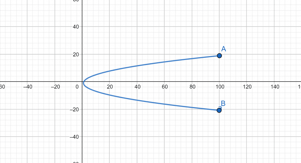
Figure 1
Example 2
Consider that there are following parametric equations:
\[\begin{matrix} x = 5 \cos t & y = 2 \sin t & 0 \leq t \leq 2 \pi \end{matrix} \]
Find the solution to these parametric equations corresponding to the parameter $t$ in the given range.
Solution
In this example, we similarly start at the Arbitrary set of parameter data based on its nature. Where Integer Data corresponds to integer values to be fed into the system, when using Angular Data, we have to rely on angles as the parametric basis. So, the angles would have to be in a range and a small size apart as this data is angular.
This is done as follows:
\[\begin{matrix}t & x & y \\ 0 & 5 & 0\\ \frac{\pi}{2} & 0 & 2\\ \pi & -5 & 0\\ \frac{3\pi}{2} & 0 & -2 \\ 2\pi & 5 & 0 \end{matrix}\]
And the parametric plot for these equations created is as follows:
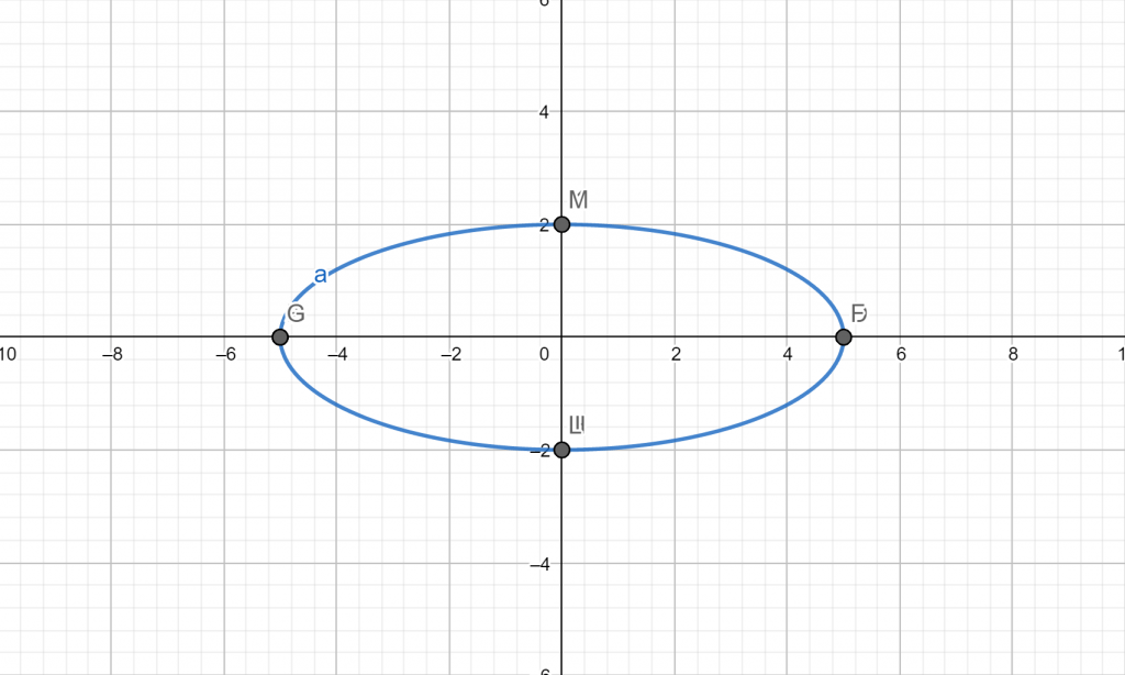
Figure 2
Example 3
Now we consider another set of parametric equations:
\[\begin{matrix} x = \sin^2 t & y = 2 \cos t & 0 \leq t \leq 2 \pi \end{matrix} \]
Find the solution to said equations associated with the parameter $t$ representing an angle.
Solution
This is another example where an arbitrary set of parameter data is built based on its nature. We know that for this example, the parameter under question $t$ corresponds to angle, so we use angular data in the range $0 – 2\pi$. Now we solve this further using these data points taken.
This is proceeds as follows:
\[\begin{matrix}t & x & y \\ 0 & 0 & 2\\ \frac{\pi}{2} & 1 & 0\\ \pi & 0 & -2\\ \frac{3\pi}{2} & 1 & 0 \\ 2\pi & 0 & 2 \end{matrix}\]
And the parametric curve for this can be drawn as such:
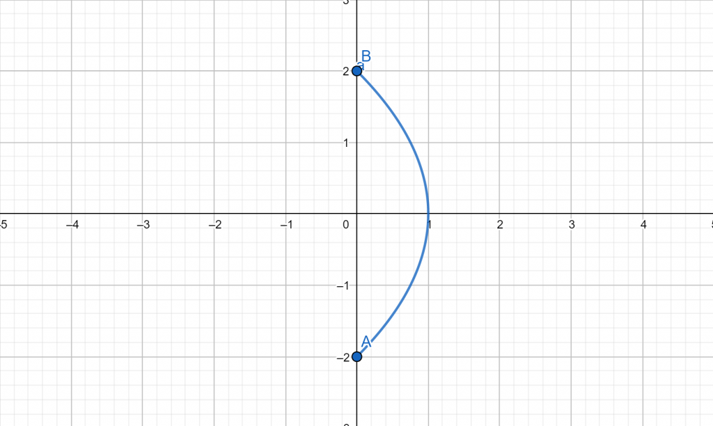
Figure 3
All images/graphs are created using GeoGebra.