JUMP TO TOPIC
Second Order Differential Equation Calculator + Online Solver With Free Steps
The Second Order Differential Equation Calculator is used to find the initial value solution of second order linear differential equations.
The second order differential equation is in the form:
L(x)y´´ + M(x)y´ + N(x) = H(x)
Where L(x), M(x) and N(x) are continuous functions of x.
If the function H(x) is equal to zero, the resulting equation is a homogeneous linear equation written as:
L(x)y´´ + M(x)y´ + N(x) = 0
If H(x) is not equal to zero, the linear equation is a non-homogeneous differential equation.
Also in the equation,
\[ y´´ = \frac{ d^{ \ 2} \ y }{ d \ x^{2} } \]
\[ y´ = \frac{ d \ y }{ d \ x } \]
If L(x), M(x), and N(x) are constants in the second order homogeneous differential equation, the equation can be written as:
ly´´ + my´ + n = 0
Where l, m, and n are constants.
A typical solution for this equation can be written as:
\[ y = e^{rx} \]
The first derivative of this function is:
\[ y´ = re^{rx} \]
The second derivative of the function is:
\[ y´´ = r^{2} e^{rx} \]
Substituting the values of y, y´, and y´´ in the homogeneous equation and simplifying, we get:
$l r^{2}$ + m r + n = 0
Solving for the value of r by using the quadratic formula gives:
\[ r = \frac{ – \ m \pm \sqrt{ m^{2} \ – \ 4 \ l \ n } } { 2 \ l } \]
The value of ‘r’ gives three different cases for the solution of the second-order homogeneous differential equation.
If the discriminant $ m^{2}$ – 4 l n is greater than zero, the two roots will be real and unequal. For this case, the general solution for the differential equation is:
\[ y = c_{1} \ e^{ r_{1} \ x} + c_{2} \ e^{ r_{2} \ x} \]
If the discriminant is equal to zero, there will be one real root. For this case, the general solution is:
\[ y = c_{1} \ e^{ r x } + c_{2} \ x e^{ r x } \]
If the value of $ m^{2}$ – 4 l n is less than zero, the two roots will be complex numbers. The values of r1 and r2 will be:
\[ r_{1} = α + βί \ , \ r_{1} = α \ – \ βί \]
In this case, the general solution will be:
\[ y = e^{ αx } \ [ \ c_{1} \ cos( βx) + c_{2} \ sin( βx) \ ] \]
The initial value conditions y(0) and y´(0) specified by the user determine the values of c1 and c2 in the general solution.

What Is a Second Order Differential Equation Calculator?
The Second Order Differential Equation Calculator is an online tool that is used to calculate the initial value solution of a second order homogeneous or non-homogeneous linear differential equation.
How To Use the Second Order Differential Equation Calculator
The user can follow the steps given below to use the Second Order Differential Equation Calculator.
Step 1
The user must first enter the second-order linear differential equation in the input window of the calculator. The equation is of the form:
L(x)y´´ + M(x)y´ + N(x) = H(x)
Here L(x), M(x), and N(x) can be continuous functions or constants depending upon the user.
The function ‘H(x)’ can be equal to zero or a continuous function.
Step 2
The user must now enter the initial values for the second-order differential equation. They should be entered in blocks labeled, “y(0)” and “y´(0)”.
Here y(0) is the value of y at x=0.
The value y´(0) comes from taking the first derivative of y and putting x=0 in the first derivative function.
Output
The calculator displays the output in the following windows.
Input
The input window of the calculator shows the input differential equation entered by the user. It also displays the initial value conditions y(0) and y´(0).
Result
The Result’s window shows the initial value solution obtained from the general solution of the differential equation. The solution is a function of x in terms of y.
Autonomous Equation
The calculator displays the autonomous form of the second-order differential equation in this window. It is expressed by keeping the y´´ on the left-hand side of the equation.
ODE Classification
ODE stands for Ordinary Differential Equation. The calculator displays the classification of differential equations entered by the user in this window.
Alternate Form
The calculator shows the alternate form of the input differential equation in this window.
Plots of the Solution
The calculator also displays the solution plot of the differential equation solution in this window.
Solved Examples
The following example is solved through the Second Order Differential Equation Calculator.
Example 1
Find the general solution for the second-order differential equation given below:
y´´ + 4y´ = 0
Find the initial value solution with the initial conditions given:
y(0) = 4
y´(0) = 6
Solution
The user must first enter the coefficients of the given second-order differential equation in the calculator’s input window. The coefficients of y´´, y´, and y are 1, 4, and 0 respectively.
The equation is homogeneous as the right-hand side of the equation is 0.
After entering the equation, the user must now enter the initial conditions as given in the example.
The user must now “Submit” the input data and let the calculator compute the differential equation solution.
The output window first shows the input equation interpreted by the calculator. It is given as follows:
y´´(x) + 4 y´(x) = 0
The calculator computes the differential equation solution and shows the Result as follows:
\[ y(x) = \frac{11}{2} \ – \ \frac{ 3 e^{- \ 4x} }{ 2 } \]
The calculator displays the Autonomous Equation as follows:
y´´(x) = – 4y´(x)
The ODE classification of the input equation is a second-order linear ordinary differential equation.
The Alternate Form given by the calculator is:
y´´(x) = – 4y´(x)
y(0) = 4
y´(0) = 6
The calculator also displays the solution plot as shown in figure 1.
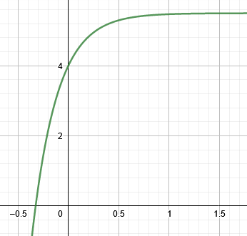
Figure 1
All the images are created using Geogebra.