JUMP TO TOPIC
Taylor Series Calculator + Online Solver With Steps
The online Taylor Series Calculator helps you find the expansion and form the Taylor Series of a given function. You can find the step-by-step solution for any given function using this calculator.
Taylor Series is the function that we get by summation of infinite terms. These terms are the derivatives of the given functions at a single point only.
This calculator also helps you find the Maclaurin series of functions. One can find the Maclaurin series by putting the point equal to zero.

What Is the Taylor Series Calculator?
Taylor Series Calculator is an online calculator that gives the expansion of a function at one point.
It is a handy tool for determining infinite sums and partial sums of functions and it extends the idea of linearization.
The process of finding the solution or expansion is lengthy and complex but it is the core of mathematics and calculus. The expression of this series reduces many lengthy and complex mathematical proofs.
Also, the Taylor series has many practical applications in physics like it can be used in the analysis of the power flow of the electrical power systems. Taylor Series is represented by the following expression:
\[ f(x) = f(a) + \frac{f’(a)}{1!}(x – a) + \frac{f’’(a)}{2!}(x – a)^{2} + \frac{f’’’(a)}{3!}(x – a)^{3} + . . . \]
The above expression is the general form of the Taylor series for the function f(x). In this equation f’(a), f’’(a) represents the derivative of the function at a specific point a. To determine the Maclaurin Series just replace point ‘a’ with zero.
How To Use the Taylor Series Calculator?
You can use the Taylor Series Calculator by entering the function, variable, and point in the given respective spaces.
The procedure for using the Taylor series calculator is made user-friendly. You just need to follow the simple steps mentioned below.
Step 1
Enter the function whose Taylor series you wish to find. For example, it can be any trigonometric like sin(x) or algebraic function such as polynomial. The function is represented by f(x).
Step 2
Enter the name of your variable. The expression entered in the above step should be the function of this variable. Also, the Taylor series is calculated using this variable.
Step 3
Set your desired point. This point can vary from one problem to another problem.
Step 4
Now, insert the order of your equation in the given last space.
Result
Click ‘submit’ to start the calculation. Once you click the button a window will pop up showing the results in a few seconds. If you want to see more detailed steps, click on the ‘more’ button.
Following is the formula used to find the Taylor series manually:
\[ F(x) = \sum_{n=0}^{\infty} (\frac{f^{n}(a)}{n!} (x – a)^n) \]
How Does the Taylor Series Calculator Work?
This calculator works by finding the derivatives of terms and simplifying them. Before we proceed we should know about some basic terms like derivatives, order of the polynomial, factorial, etc.
What Are Derivatives?
Derivatives are simply the instantaneous rate of change of any quantity. The derivative of the function is the slope of the line tangent to the curve at any value of a variable.
For example, if the rate of change for the variable y is found with respect to the variable x. Then the derivative is denoted by the term ‘dy/dx’ and the general formula for calculating the derivative is:
\[ \frac{dy}{dx} = \lim_{a \to 0} \frac{f(x + a) – f(x)}{a} \]
What Is a Factorial?
Factorial is the product of any whole number with all the whole numbers until 1. For example, the factorial of 5 will be 5.4.3.2.1 which equals 120. It is represented as 5!
What Is the Order of an Equation?
The highest order of the terms in an equation is known as the order of the equation. For example, if the high order in a term is 2 so the order of the equation will be 2 and it will be called the second order equation.
What Is Summation?
Summation is the operation of adding multiple terms together. The Sigma ($\sum$) sign is used to represent summation. It is generally used to add components of discrete signals.
What Is Power Series?
Power series is a series of any polynomial which has an infinite number of terms. The Taylor series is an advanced form of power series. For example, the power series looks like the following expression.
\[ 1+y+y^{2}+y^{3}+y^{4} + … \]
Method of Calculation
The calculator asks the user to enter the given data that have been explained in the previous section. After clicking the submit button, it shows the output in a few seconds with detailed steps.
Here are the simplified steps that are used to get the final results.
Finding Derivatives
Finding the derivatives of the functions is the first step. The calculator finds the derivatives of terms according to their order. Like initially it calculates the first-order derivative, then the second, and so on depending on the order of the equation.
Putting Values
In this step, it replaces the variable with the point at which the value is required. This is a simple step in which the function is expressed in the terms of the value of the point.
Simplification
Now, the calculator puts the results from the above step in the general formula of the Taylor Series. In this step, after putting the values it simplifies the expression through simple mathematical steps like taking factorial, etc.
Summation
Finally, the calculator adds a summation sign and gives the result. The summation is helpful if we want to determine the interval on convergence or some specific values of the variable where the Taylor series converges.
Plotting Graphs
It’s difficult and complex to draw the graph manually. But this calculator shows an approximate graph for the given variable up to order 3.
More Detail About Taylor Series
In this section, we will discuss the tailor series from its historic view, the applications of the Taylor Series, and its limitations.
Brief History of the Taylor Series
Taylor is the name of the scientist who introduced this series in 1715. His complete name is Brook Taylor.
In the mid-1700s another scientist Colin Maclaurin used the Taylor series extensively in a special case in which zero is taken as the point of derivatives. This is known after his name as the Maclaurin series.
Applications of the Taylor Series
- It helps in evaluating definite integrals as some functions may not have their antiderivative.
- Taylor Series can help understand the behavior of the function in its specific domain.
- The growth of functions can also be understood through the Taylor series.
- Taylor Series and Maclaurin series are used to find the approximate value of the Lorentz factor in special relativity.
- The basics of pendulum motion are also derived through the Taylor series.
Limitations of the Taylor Series
- The most common limitation of the Taylor Series is that it becomes more and more complex as we move to the further steps it becomes difficult to handle it.
- Two types of errors are there that may affect whole calculations that are round-off error and truncation error. Away from the point of expansion, the truncation error grows rapidly.
- Calculations are lengthy and time-consuming if we do them by hand.
- This method is not certain for the solution of Ordinary Differential Equations.
- It is usually not much efficient compared to curve fitting.
Solved Examples
Now let’s solve some examples to understand the working of the Taylor Series calculator. The examples are described below:
Example 1
Find the Taylor Series of f(x) = $e^{x}$ at x=0 and order is equal to 3.
Solution
It finds the first three derivatives of the input equation that are given as:
\[ f’(x) = e^{x}, \, f’’(x) = e^{x}, \,f’’’(x) = e^{x} \]
As the function is of exponential type, all of the derivatives are equal.
At point x=0, we get the following values for each derivative.
f’(0) = f’’(0) = f’’’(0) = 1
Then the values are inserted in the general form of the Taylor series.
\[ f(x) = f(0) + \frac{f’(0)}{1!}(x – 0) + \frac{f’’(0)}{2!}(x – 0)^{2} + \frac{f’’’(0)}{3!}(x – 0)^{3} + . . . \]
Further reduce the expression by solving it.
\[ f(x) = f(0) + \frac{f’(0)}{1!}(x) + \frac{f’’(0)}{2!}(x)^{2} + \frac{f’’’(0)}{3!}(x)^{3} + . . . \]
\[ e^{x} = 1 + x(1) + \frac{x^{2}}{2!}(1) + \frac{x^{3}}{3!}(1) \]
At last, it gives the following result which is the final solution to the problem.
\[ e^{x} = 1 + x + \frac{x^{2}}{2!} + \frac{x^{3}}{3!} \]
Graph
The graph in figure 1 is the approximation of the series at x=0 up to order 3.
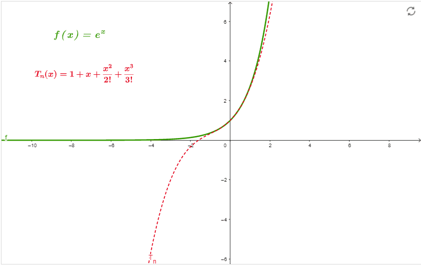
Figure 1
Example 2
Find the Taylor Series for f(x) = $x^3$ − 10$x^2$ + 6 at x = 3.
Solution
The answer is briefly described in steps. The derivative calculation for the function is given below. Besides calculating derivatives, the values of derivatives at the given point are also calculated.
\[ f(x) = x^{3} – 10 x^{2} + 6 \Rightarrow f(3) = – 57 \]
\[ f’(x) = 3x^{2} – 20 x + 6 \Rightarrow f’(3) = 33 \]
f’’(x) = 6 x – 20 x + 6 $\Rightarrow$ f’’(3) = -2
f’’’(x) = 6 $\Rightarrow$ f’’’(3) = 6
Now putting values in the general formula for the Taylor series,
\[ x^{3} – 10 x^{2} + 6 = \sum_{n=0}^{\infty} (\frac{f^{n}(3)}{n!} (x – 3)^n) \]
\[ = f(3) + \frac{f’(3)}{1!}(x – 3) + \frac{f’’(3)}{2!}(x – 3)^{2} + \frac{f’’’(3)}{3!}(x – 3)^{3} + 0 \]
\[ = f(3) + f’(3)(x – 3) + \frac{f’’(3)}{2!}(x – 3)^{2} + \frac{f’’’(3)}{3!}(x – 3)^{3} + 0 \]
\[ = – 57 – 33(x – 3) – (-3)^{2} + (x – 3)^{3} \]
Graph
The series can be visualized in the following graph in the below figure.
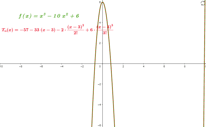
Figure 2
All the Mathematical Images/Graphs are created using GeoGebra.