JUMP TO TOPIC
Riemann Sum Calculator + Online Solver With Free Steps
The Riemann Sum Calculator approximates the value of an integral with the Riemann Sum Approximation method. It requires the function for integration, the interval over which to evaluate it, and the number of sub-intervals for the approximation.
The calculator additionally allows choosing between three specific types of the Riemann sum: left, middle/midpoint, and right.
The calculator does not support multi-variable functions. Therefore, you must use single variable functions, but you may use constants defined as variables. To enter a constant as a variable, use the commonly used characters denoting constants such as a, b, c, etc.
However, an input like “(xy)^2” is considered a multi-variable function by the calculator resulting in no output.

What Is the Riemann Sum Calculator?
The Riemann Sum Calculator is an online tool that evaluates the integral of a function over some interval of values using a discrete summation (finite sum) of areas of rectangular regions based on the function curve. This approach to integral estimation is termed the Riemann Sum Approximation.
The calculator interface consists of one drop-down menu and four text boxes. The drop-down menu offers three options that define the type of Riemann sum approximation used to calculate the result: “left,” “right,” and “midpoint.”
The text boxes are labeled:
- “Riemann sum of”: The expression of the specific function for which to approximate the integral. It must be a function of one variable. However, it may contain constants as variables.
- “From”: The start point for evaluation of the Riemann sums. In other words, the initial value of the integral interval.
- “To”: The endpoint for the evaluation of the Riemann sums. It is the final value of the integral interval.
- “With [text box] subintervals”: The number of sub-intervals to use for the Riemann sum approximation. The larger this specific number, the more accurate the approximation, but at the cost of more computation time.
How To Use the Riemann Sum Calculator?
You can use the Riemann Sum Calculator to approximate the integral of a function over a closed interval by entering the function’s expression, the start and end points of the closed interval, the type of Riemann sum approximation, and the number of sub-intervals (rectangles) to use in the process.
Suppose you want to find the middle Riemann sum approximation for the integral of the function f(x) = 2abx$^\boldsymbol{\mathsf{2}}$ over the interval x = [0, 1] using a total of ten sub-intervals. The step-by-step guidelines to solve this with the calculator are shown below.
Step 1
Make sure the function contains a single variable and all constant variables are termed a, b, c, etc. The example has two constant variables, a and b, which is fine.
Step 2
From the dropdown menu labeled “compute,” choose which type of Riemann sum you want to use. In this case, select the “midpoint” option.
Step 3
Enter the function’s specific expression in the text box labeled “Riemann sum of.” For this example, enter “2abx^2” without quotes.
Step 4
Enter the closed interval of integration in the appropriate text boxes labeled “From” (initial value) and “to” (final value). Since the example has the integral interval [0, 1], enter “0” and “1” in these fields.
Step 5
Enter the number of sub-intervals for the approximation into the final text box labeled “with [text box] subintervals.” Type “10” in the text box for the example.
Results
The results show in a pop-up dialogue box with two sections:
- Result: This section displays the value of the Riemann sum approximation. For the example, the result here is “0.665ab”.
- Exact Integral Result: This section shows the result of the exact integral calculation, allowing us to evaluate the accuracy of the approximation. For the example, the resulting value is (2/3)ab $\boldsymbol{\approx}$ 0.6667ab which is quite close to the approximated value.
In both sections, you can choose to increase the number of decimal places shown using the “More digits” prompt.
How Does the Riemann Sum Calculator Work?
The Riemann Sum Calculator works by using the following formula:
\[ \int_a^b f(x)\,dx \approx S = \sum_{k=1}^n f(x=x_k) \left( \Delta x \right) \tag*{$(1)$} \]
A curve defined by f(x) over a closed interval [a, b] can be split into n rectangles (sub-intervals) each of length $\frac{b-a}{n}$ with endpoints [i$_\mathsf{k}$, f$_\mathsf{k}$]. The height of the kth rectangle then equals the value of the function at one of the endpoints of the kth sub-interval [i$_\mathsf{k}$, f$_\mathsf{k}$].
The area of the kth rectangle is then:
\[ R_k = f(x=x_k) \left( \frac{b-a}{n} \right) \,\, \text{where} \,\, x_k \, \in \, [\,i_k,\, f_k\,] \]
Where $\frac{b-a}{n}$ is usually termed $\Delta$x and also equals f$_\mathsf{k}$ – i$_\mathsf{k}$. Then if we add all the rectangles together, we get the Riemann sum as in equation (1):
\[ S= \sum_{k=1}^n f(x=x_k) \left( \Delta x \right) \]
The choice of x$_\mathsf{k}$ for the calculations leads to the various types of Riemann sums. The ones provided by the calculator are:
- Left Riemann Sum: Use the starting point of each sub-interval such that x$_\mathsf{k}$ = i$_\mathsf{k}$.
- Right Riemann Sum: Use the endpoint of each sub-interval such that x$_\mathsf{k}$ = f$_\mathsf{k}$.
- Middle Riemann Sum: Use the midpoint of each sub-interval such that $x_k = \frac{f_k-i_k}{2}$.
Significance
The Riemann sum approximation is a fundamental part of Calculus. It approximates integrals of continuous curves as a finite sum of areas of regular shapes such as rectangles.
Thus, it essentially defines the concept of an integral. If the number of sub-intervals approaches infinity, the Riemann sum approaches the Riemann integral, which is the limit of the Riemann sum as n to $\infty$. This proves that the integral of a function is the area under the function’s curve.
Additionally, while some functions allow a simple formulation of the integral (known as a function having an explicit integral), this is not true for all of them. In such cases, one cannot solve the integral directly and must approximate it somehow (e.g., with Riemann sums).
Solved Examples
Example 1
Find the area of the curve x$^\mathsf{2}$ for the interval [-1, 1]. Use the middle Riemann sum approximation with four sub-intervals and compare it with the exact integral value.
Solution
Given that:
f(x) = x$^\mathsf{2}$ for x = [-1, 1]
Middle Riemann Sum With Four Subintervals
A quick visualization of what we are about to do:
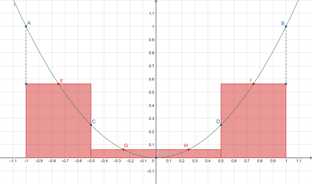
Figure 1
Where A, B, C, D, and O represent the points on the partitioned curve while F, G, H, and I respectively show the midpoints of the sub-intervals [A, C], [C, O], [O, D], and [D, B]. We are going to sum the areas of the rectangles in red!
Interval to Sub-intervals
First, we divide the interval into four sub-intervals. Let the complete integral interval length be ‘l‘ with endpoints a and b, then:
\[ l = \left \vert \, \text{final point}-\text{initial point} \, \right \vert \]
\[ \Rightarrow \, l = \left \vert \, b-a \, \right \vert = \left \vert \, 1-(-1) \, \right \vert = 2 \]
Dividing l by n=4, we get the length for each sub-interval $\Delta x$:
\[ \Delta x = \frac{b-a}{n} = \frac{l}{4} = \frac{2}{4} = \frac{1}{2} = 0.5 \]
Generally, the $k^{th}$ sub-interval’s range $I_k$ is then:
\[ I_k = \left[ \, i_k, \, f_k \, \right] \tag*{$k=1,\, 2,\, 3,\, \ldots,\, n$} \]
\[ \left[ \, i_k, \, f_k \, \right] = \left\{ \begin{array}{rcl} \left[\, a, \, a + \Delta x \, \right] & \text{for} & k = 1 \\ \left[ \, f_{k-1}, \, f_{k-1} + \Delta x \, \right] & \text{for} & k > 1 \\ \left[ b-\Delta x, \, b \right] & \text{for} & k = n \end{array} \right. \]
Note how the endpoint for $I_k$ is the start point for $I_{k+1}$. Thus, we can specify a general sequence for the points representing the endpoints of n sub-intervals:
\[ A = \left\{ a,\, a + \Delta x,\, a + 2\Delta x,\, \ldots,\, a + (n-1)\Delta x,\, b \right\} \]
Where $b = a + n\Delta x$. In the above sequence, every consecutive pair of values forms a sub-interval. For example, $(a+\Delta x,\, a+2\Delta x)$ forms one such pair representing the second sub-interval.
In our case, using the above formulations gets us the following ranges for the four sub-intervals:
\[ \begin{array}{ccccc} I_1 & = & \left[ -1.0,\, -1.0+0.5 \right] & = & \left[ -1.0,\, -0.5 \right] \\ I_2 & = & \left[ -0.5,\, -0.5+0.5 \right] & = & \left[ -0.5,\, 0.5 \right] \\ I_3 & = & \left[ 0.0,\, 0.0+0.5 \right] & = & \left[ 0.0,\, 0.5 \right] \\ I_4 & = & \left[ 0.5,\, 0.5+0.5 \right] & = & \left[ 0.5,\, 1.0 \right] \end{array} \]
And the sequence of endpoints for the sub-intervals:
A = { -1, -0.5, 0, 0.5, 1 }
Calculating the Riemann Sum
Since we are using the middle Riemann sums, we need to evaluate the function at the midpoint of each sub-interval and multiply it with the length of the sub-intervals. That is, we require the following:
\[ \int_{-1}^1 x^2dx \approx S = \Delta x \sum_{k\,=\,1}^{n\,=\,4} f (\underbrace{a + (k-1)\Delta x}_{\substack{\text{start point of} \\ \text{k$^\text{th}$ sub-interval $i_k$}}} + 0.5\Delta x ) \]
Where 0.5$\Delta$x represents half the sub-interval length. It is added to the initial point i$_\mathsf{k}$ to get to the midpoint of the interval. Thus, f(a + (k-1) $\Delta$x + 0.5$\Delta$x) represents the function value (height of k$^\textsf{th}$ rectangle) at the k$^\textsf{th}$ sub-interval midpoint. Equivalently:
\[ S = \Delta x \sum_{k\,=\,1}^{n\,=\,4} f \left( A_k + 0.5\Delta x \right) \]
Knowing that $0.5\Delta x$ = 0.5(0.5) = 0.25, we can solve the above equation to get the following result:
\[ S = \Delta x \left\{ f(x=-1+0.25) + f(x=-0.5+0.25) + f(x= 0+0.25) + f(x=0.5+0.25) \right\} \]
\[ S = 0.5 \left\{ (-0.75)^2 + (-0.25)^2 + 0.25^2 + 0.75^2 \right\} \]
\[ \Rightarrow \, S = 0.5 \left( 1.25 \right) = \mathbf{\frac{5}{8}} = \mathbf{0.625} \]
Exact Integral Result
The integral of the function f(x) = $x^2$ is explicitly known:
\[ \int x^ndx = \frac{x^{n+1}}{n+1} + C \]
Applying this to our problem by substituting n = 2, we get the result:
\[ \int x^2dx = \frac{x^{2+1}}{2+1} = \frac{x^3}{3} \]
Evaluating the integral result over the closed interval x = [-1, 1]:
\[ \int_{-1}^1 x^2dx = \left. \frac{x^3}{3} \right \rvert_{x\,=\,-1}^{x\,=\,1} \]
\[ \int_{-1}^1 x^2dx = \frac{1^3}{3}-\frac{(-1)^3}{3} = \frac{1}{3}+\frac{1}{3} \]
\[ \Rightarrow \, \int_{-1}^1 x^2dx = \mathbf{\frac{2}{3}} \approx \mathbf{0.66667} \]
The current error is:
0.66667-0.625 = 0.04167
Increasing the number of subintervals n will help reduce it further.
All graphs/images were created with GeoGebra.