JUMP TO TOPIC
Sinusoidal Function Calculator + Online Solver With Free Steps
The Sinusoidal Function Calculator plots the trigonometric functions sin(x), cos(x), and tan(x) given the period, amplitude, vertical, and phase shift values. The calculator shows two plots: one is over a smaller range of x (zoomed in), and the other is over a larger interval of x (zoomed out).
A sinusoid or sinusoidal wave is a continuous and smooth periodic wave, representable by a sine function such as sine or cosine (hence the name, sinusoid).
One of the input parameters can be a variable (other than x). The calculator then displays a 3D plot with the function value over the z-axis. x varies over the x-axis and the variable input parameter over the y-axis. Additionally, the equivalent 2D contours are also displayed.
If there is more than one variable parameter other than x, the required plot dimensions exceed three, and the calculator does not plot anything.

What Is the Sinusoidal Function Calculator?
The Sinusoidal Function Calculator is an online tool that applies the chosen trigonometric function to the variable x using the provided values of the parameters (amplitude, period, vertical shift, phase shift). The range of values for x is chosen automatically for an appropriate visualization.
You may think of x as time t. It allows for an intuitive understanding of the results.
The calculator interface consists of one drop-down menu labeled “Function” with three trigonometric functions as options: “sin,” “cos,” and “tan.” Additionally, there are four text boxes labeled:
- A – Amplitude: The peak value of the sinusoid. Since the sin function outputs in the range [-1, 1], multiplication by the amplitude value A brings the range to [ -A, A].
- B – Period: Angular frequency $\omega = 2 \pi f$ or rate of change of function in radians per second. Specifically, if $2\pi$ represents one complete cycle at a frequency of 1 Hz (per second), then $2\pi(50)$ means fifty cycles in the same time (per second), or one cycle every $\frac{1}{50}$ = 20 ms seconds.
- C – Phase Shift: Offset of the wave along the x-axis. For example, the unit amplitude sinusoid with period $2\pi$ reaches the peak value of 1 at x = 0.25. If a phase angle of $\frac{\pi}{2}$ is subtracted from this, the sinusoid shifts right, so the new value at x = 0.25 is 0. The peak shifts to 0.5.
- D – Vertical Shift: Offset along the y-axis (function value). The entire range of the function values changes with this value since the function is periodic. For example, if the range of the function was [ -1, 1], a vertical shift of D = 1.5 would make the new range [-1+1.5, 1+1.5 ] = [ 0.5, 2.5 ].
Mathematical Notation
The calculator utilizes the simple form of a sinusoid:
amplitude x sin(angular frequency x time – phase shift) + vertical shift
Where vertical shift is also called the center amplitude. In mathematical notation, the amplitude is generally termed A, the angular frequency $\omega$, the phase shift $\varphi$, and the vertical shift as D. The equation then becomes:
f(x) = A sin($\omega$ t-$\varphi$) + D
Positive entries in the phase shift text box imply a right shift, and negative entries indicate a left shift.
How To Use the Sinusoidal Function Calculator?
You can use the Sinusoidal Function Calculator by choosing the trigonometric function to apply and entering the required parameters into their respective fields. For example, let us suppose we want to plot the following function:
f(x) = y = 0.1x sin(2 $\pi$ x-$\pi$) + 1.5
To plot this function, follow the step-by-step guidelines below.
Step 1
Compare the input expression with the form the calculator expects:
f(x) = A sin(Bx-C) + D
We can see that A (amplitude) = 0.1x, B (period) = 2 $\pi$, C (phase shift) = $\pi$, and D(vertical shift) = 1.5 for our case.
Step 2
Choose the trigonometric function you want to apply from the drop-down menu labeled “Function.” In our case, we select “sin” without the quotes.
Step 3
Enter the rest of the parameters into their respective text boxes: A, B, C, and D found in Step 1. For our example, we respectively enter “0.1x,” “2*pi,” “pi,” and “1.5” without the quotes and separating commas.
Step 4
Press the Submit button to get the resulting plots.
Results
The results are plots of the function over an automatically chosen and scaled range of values of the variable x. Note that the amplitude in our example is also a function of x, not some other variable. Therefore, the results will be 2D plots.
Solved Examples
Example 1
Given the amplitude of the sinusoid is 5 and the frequency is 50 Hz, plot its graph.
Solution
\[ \because \, \omega = 2 \pi f = 2 \pi (50) = 100 \pi\]
$\Rightarrow$ f(x) = 5 sin(100 $\pi$ . x)
$\Rightarrow$ A = 5, B = 100 $\pi$, C = 0, D = 0
The graph:
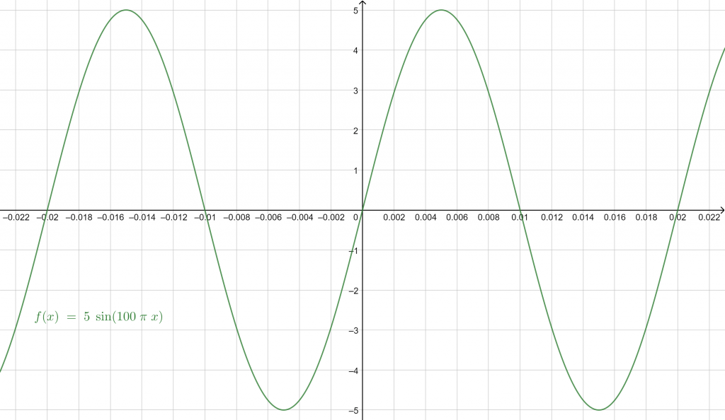
Figure 1
Example 2
For the sinusoidal function in Example 1, perform a rightwards phase shift of $\frac{\pi}{2}$ and plot it again.
Solution
The input according to the calculator’s standard sinusoidal equation:
\[ f(x) = 5 \sin(2 \pi (50) \cdot x-\frac{\pi}{2}) \]
$\Rightarrow$ \, A = 5, B = 100 $\pi$, $C = \frac{\pi}{2}$, D = 0
Note that C is positive because we require the rightwards phase shift.
The plot is then:
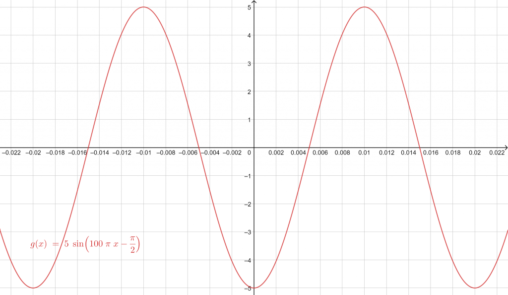
Figure 2
And the difference between the function in examples 1 and 2 can be seen by putting them side-by-side:
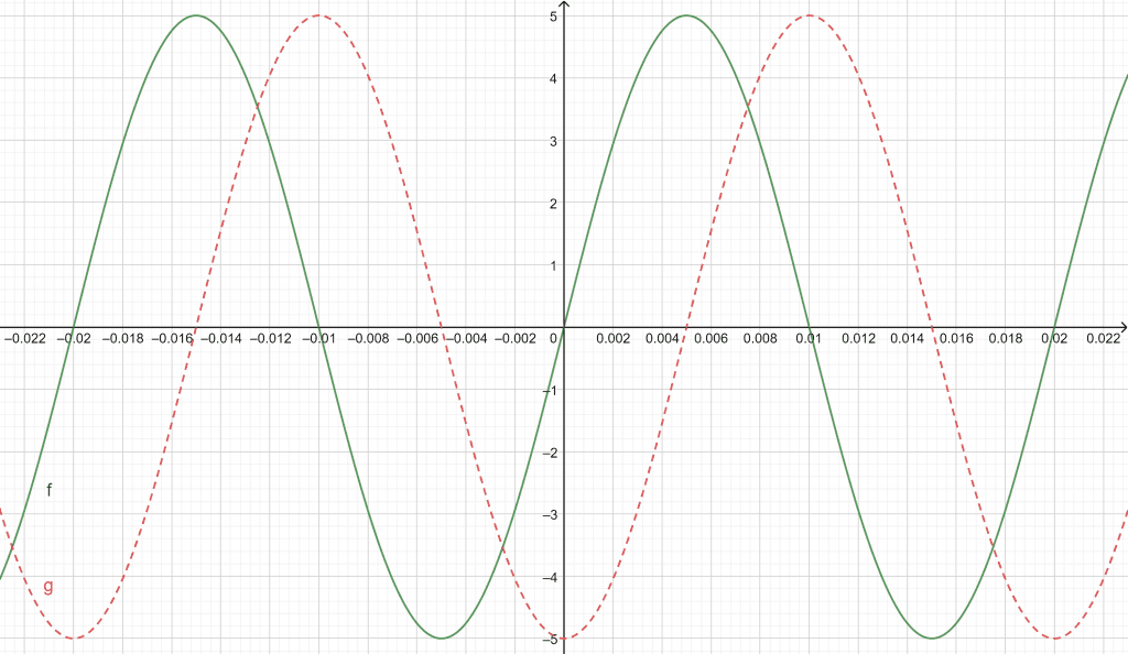
Figure 3
Example 3
Plot the sinusoidal function:
f(x) = y = 0.1x sin(2 $\pi$ x-$\pi$) + 1.5
Solution
Putting A = 0.1x, B = $\omega$ = 2 $\pi$, C = $\varphi = -\pi$, and D = 1.5 and submitting to the calculator gets us the plot:
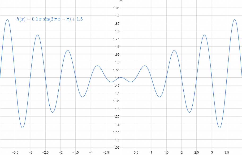
Figure 4
Example 4
Plot the sinusoidal with A = 1, $\omega = y$, $\varphi = \frac{\pi}{2}$, and D = 0 as a function of both time and y.
Solution
In the standard form:
\[ f(x, y) = \sin \left( yx-\frac{\pi}{2} \right) \]
The calculator gives the plot of the function f(x, y):
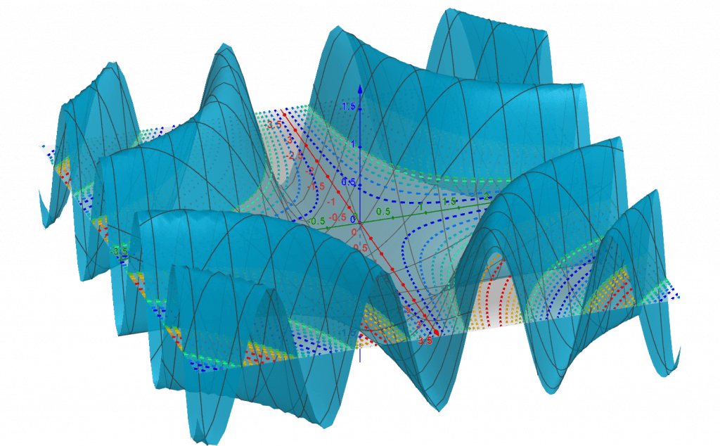
Figure 5
And the contour plot (level curves shown here):
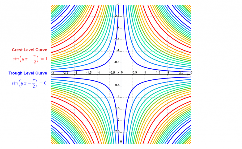
Figure 6
All images/graphs were drawn with GeoGebra.