JUMP TO TOPIC
Trapezoidal Rule Calculator + Online Solver With Free Steps
The Trapezoidal Rule Calculator estimates the definite integral of a function over a closed interval using the Trapezoidal Rule with a specified number of trapezoids (sub-intervals). The Trapezoidal rule approximates the integral by dividing the region under the function curve into n trapezoids and summing up their areas.
The calculator only supports single variable functions. Therefore, an input like “sin(xy)^2” is considered a multi-variable function by the calculator resulting in no output. Variables representing constants such as a, b, and c are also not supported.

What Is the Trapezoidal Rule Calculator?
The Trapezoidal Rule Calculator is an online tool that approximates the definite integral of a function f(x) over some closed interval [a, b] with a discrete summation of n trapezoid areas under the function curve. This approach for approximation of definite integrals is known as the Trapezoidal Rule.
The calculator interface consists of four text boxes labeled:
- “Function”: The function for which to approximate the integral. It must be a function of only one variable.
- “Number of Trapezoids”: The number of trapezoids or sub-intervals n to use for the approximation. The larger this number, the more accurate the approximation at the cost of more computation time.
- “Lower Limit”: The initial point for the summation of trapezoids. In other words, the initial value a of the integral interval [a, b].
- “Upper Limit”: The endpoint for the summation of trapezoids. It is the final value b of the integral interval [a, b].
How To Use the Trapezoidal Rule Calculator?
You can use the Trapezoidal Rule Calculator to estimate the integral of a function over an interval by entering the function, the integral interval, and the number of trapezoids to use for the approximation.
For example, suppose you want to estimate the integral of the function f(x) = x$^\mathsf{2}$ over the interval x = [0, 2] using a total of eight trapezoids. The step-by-step guidelines to do so with the calculator are below.
Step 1
Ensure the function contains a single variable and no other characters.
Step 2
Enter the function’s expression in the text box labeled “Function.” For this example, enter “x^2” without quotes.
Step 3
Enter the number of sub-intervals in the approximation into the final text box labeled “with [text box] subintervals.” Type “8” in the text box for the example.
Step 4
Enter the integral interval in the text boxes labeled “Lower Limit” (initial value) and “Upper Limit” (final value). Since the example input has the integral interval [0, 2], enter “0” and “2” in these fields.
Results
The results show in a pop-up dialogue box with just one section labeled “Result.” It contains the value of the approximated value of the integral. For our example, it is 2.6875 and therefore:
\[ \int_0^2 x^2 \, dx \approx 2.6875 \]
You can choose to increase the number of decimal places shown using the “More digits” prompt at the top-right corner of the section.
How Does the Trapezoidal Rule Calculator Work?
The Trapezoidal Rule Calculator works by using the following formula:
\[ \int_a^b f(x)dx \approx S = \sum_{k\,=\,1}^n \frac{f(x_{k-1}) + f(x_k)}{2} \Delta x \tag*{$(1)$} \]
Definition and Understanding
A trapezoid has two parallel sides opposite each other. The other two sides are not parallel and generally intersect the parallel ones at an angle. Let the length of the parallel sides be l$_\mathsf{1}$ and l$_\mathsf{2}$. Assuming the perpendicular length between the parallel lines is h, then the trapezoid’s area is:
\[ A_{\text{trapezoid}} = \frac{1}{2}h(l_1+l_2) \tag*{$(2)$} \]
A curve defined by f(x) over a closed interval [a, b] can be split into n trapezoids (sub-intervals) each of length $\Delta$x = (b – a) / n with endpoints [i$_\mathsf{k}$, f$_\mathsf{k}$]. The length $\Delta$x represents the perpendicular distance h between parallel lines of the trapezoid in equation (2).
Moving on, the length of the k$^\mathsf{th}$ trapezoid’s parallel sides l$_\mathsf{1}$ and l$_\mathsf{2}$ then equals the value of the function at the extreme ends of the k$^\mathsf{th}$ sub-interval, that is l$_\mathsf{1}$ = f(x=i$_\mathsf{k}$) and l$_\mathsf{2}$ = f(x=f$_\mathsf{k}$). The area of the k$^\mathsf{th}$ trapezoid is then:
\[ T_k = \frac{1}{2}\Delta x \left( f(i_k) + f(f_k) \right) \]
If we express the sum of all n trapezoids, we get the equation in (1) with x$_\mathsf{k-1}$ = i$_\mathsf{k}$ and x$_\mathsf{k}$ = f$_\mathsf{k}$ in our terms:
\[ S = \frac{\Delta x}{2} \sum_{k\,=\,1}^n f(i_k) + f(f_k) \tag*{(3)} \]
Equation (1) is equivalent to the average of the left and right Riemann sums. Hence the method is often considered a form of a Riemann sum.
Solved Examples
Example 1
Find the area of the curve sin(x$^\mathsf{2}$) for the interval [-1, 1] in radians.
Solution
Given that:
\[ f(x) = \sin(x^2) \quad \text{for} \quad x = [-1, \,1] \]
The integral for this function is tricky to calculate, requiring complex analysis and involving Fresnel integrals for a complete derivation. However, we can approximate it with the trapezoidal rule!
Here’s a quick visualization of what we are about to do:
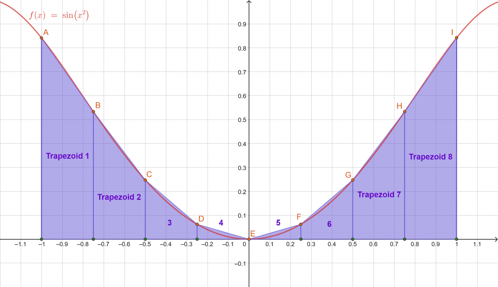
Figure 1
Interval to Sub-intervals
Let us set the number of trapezoids n = 8, then the length of each sub-interval corresponding to a trapezoid’s height h (length between two parallel segments) is:
\[ h = \Delta x = \frac{b-a}{n} = \frac{2}{8} = 0.25 \]
So the sub-intervals I$_\mathsf{k}$ = [i$_\mathsf{k}$, f$_\mathsf{k}$] are:
\[ \begin{array}{ccccc} I_1 & = & \left[ -1.0,\, -1.0+0.25 \right] & = & \left[ -1.00,\, -0.75 \right] \\ I_2 & = & \left[ -0.75,\, -0.75+0.25 \right] & = & \left[ -0.75,\, -0.50 \right] \\ I_3 & = & \left[ -0.50,\, -0.50+0.20 \right] & = & \left[ -0.50,\, -0.25 \right] \\ I_4 & = & \left[ -0.25,\, -0.25+0.25 \right] & = & \left[ -0.25,\, 0.00 \right] \\ I_5 & = & \left[ 0.00,\, 0.00+0.25 \right] & = & \left[ 0.00,\, 0.25 \right] \\ I_6 & = & \left[ 0.25,\, 0.25+0.25 \right] & = & \left[ 0.25,\, 0.50 \right] \\ I_7 & = & \left[ 0.50,\, 0.50+0.25 \right] & = & \left[ 0.50,\, 0.75 \right] \\ I_8 & = & \left[ 0.75,\, 0.75+0.25 \right] & = & \left[ 0.75,\, 1.00 \right] \end{array} \]
Applying the Trapezoidal Rule
Now we can use the formula from equation (3) to get the result:
\[ S = \frac{\Delta x}{2} \sum_{k\,=\,1}^8 f(i_k) + f(f_k) \]
To save screen space, let us separate the $\sum_\mathsf{k\,=\,1}^\mathsf{8}$ f(i$_\mathsf{k}$) + f(f$_\mathsf{k}$) into four parts as:
\[ s_1 = \sum_{k\,=\,1}^2 f(i_k) + f(f_k) \,\, , \,\, s_2 = \sum_{k\,=\,3}^4 f(i_k) + f(f_k) \]
\[ s_3 = \sum_{k\,=\,5}^6 f(i_k) + f(f_k) \,\, , \,\, s_4 = \sum_{k\,=\,7}^8 f(i_k) + f(f_k) \]
Evaluating them separately (be sure to use radian mode on your calculator):
\[ s_1 = \{f(-1) + f(-0.75)\} + \{f(-0.75) + f(-0.5)\} \]
\[ \Rightarrow s_1 = 1.37477 + 0.78071 = 2.15548\]
\[ s_2 = \{f(-0.5) + f(-0.25)\} + \{f(-0.25) + f(0)\} \]
\[ \Rightarrow s_2 = 0.30986 + 0.06246 = 0.37232 \]
\[ s_3 = \{f(0) + f(0.25)\} + \{f(0.25) + f(0.5)\} \]
\[ \Rightarrow s_3 = 0.06246 + 0.30986 = 0.37232 \]
\[ s_4 = \{f(0.5) + f(0.75)\} + \{f(0.75) + f(1)\} \]
\[ \Rightarrow s_4 = 0.78071 + 1.37477 = 2.15548 \]
\[ \therefore \, s_1 + s_2 + s_3 + s_4 = 5.0556 \]
\[ \Rightarrow \sum_{k\,=\,1}^8 f(i_k) + f(f_k) = 5.0556 \]
Putting this value into the original equation:
\[ S = \frac{0.25}{2} (5.0556) = \frac{5.0556}{8} = 0.63195 \]
\[ \Rightarrow \int_{-1}^1\sin(x^2)\,dx \approx S = \mathbf{0.63195} \]
Error
The results are close to the known exact integral value at $\approx$ 0.6205366. You can improve the approximation by increasing the number of trapezoids n.
All graphs/images were created with GeoGebra.