Normal Distribution|Definition & Meaning

Moreover, it has the potential to approximate both these probability distributions, supporting the use of the term “normal” as the most commonly used.

Bell Curve 

The Bell Curve is an example of the Normal Distribution. Data can be dispersed (spread out) in the following way. The purple distribution depicts some data that closely but needs to follow it (that is ok) entirely. It is symmetric around the mean, implying that values close to the mean happen more frequently than far away.

Figure 1 below shows the bell curve for the normal distribution.

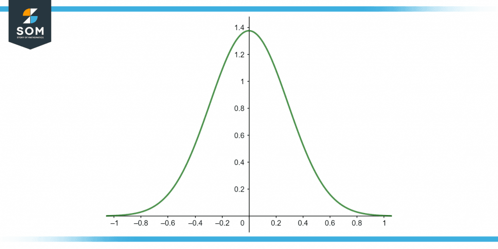
Figure 1 – Representation of a normal distribution.

The Formula for Normal Distribution

Here, x is the variable’s value, f(x) is the probability density function, mu is the mean, and sigma is the standard deviation.

The empirical rule of normal distributions specifies where the majority of the information in a normally distributed will appear as follows:

• 68.2% of the data will fall between +/-1 mean difference of a mean, 
• 95.4% would fall between +/-2 standard deviations, and 
• 99.7% will lie around +/-3 standard deviations.

All data points falling outside the three standard deviations (3) are considered unusual.

Figure 2 below shows the normal distribution’s probability density function.

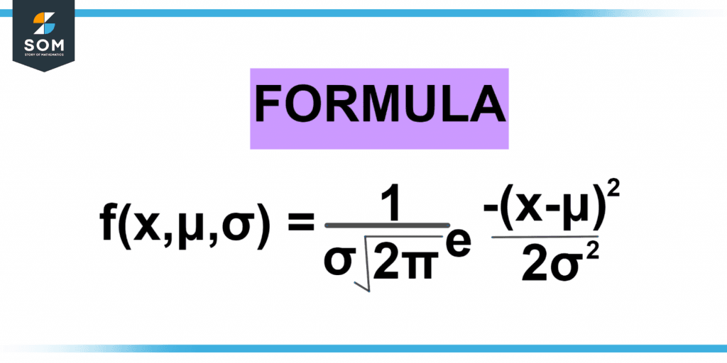
Figure 2 – Formula for normal distribution.

Normal Distribution Properties

The following are some of the essential features of the normal distribution:

• A normal distribution’s mean, median, and mode are all equal. (For example, Mean = Median = Mode).
• The whole area beneath the curve must equal one.
• At the center, a normally distributed curve ought to be symmetric.
• Precisely half of the values should be on the right of the center, and exactly half should be on the left.
• The standard deviation and mean should be used to define the normal distribution.
• The normal distribution graph can only have one peak. (In other words, Unimodal)
• The curve approaches the x-axis but never touches it and moves away from the median.

Normal Distribution Parameters

In a normal distribution, it is not necessary to calculate the mean, mode, & median separately since they are the same. These figures represent the distribution’s pinnacle or peak. The remaining values in the distribution then fall symmetrically around the mean. The standard deviation expresses the range of the mean.

The mean and standard deviation are the only parameters used to define a normal distribution.

Mean

The mean is the highest value in the middle of a bell curve. All of the other values within the distribution cluster are within it or are relatively far away. Changing the average mean on the graph causes the entire curve to move to the left or right along the x-axis. Its symmetry, however, will be preserved.

Standard Deviation

The standard deviation is the variability of dispersion or the measurement of its variability. The distribution is explained by a bell curve, which illustrates how far other numbers deviate from the mean. It also denotes the average difference between the mean and the observations.

Even when the standard deviation is changed, the dispersion of the data around the mean changes. A lower deviation severely limits the distribution by decreasing the range.

In contrast, a more significant deviation broadens the distribution by raising the spread as the distribution widens, and the chance of values deviating from the mean increases.

Normal Distribution Standard Deviation

Any high standard deviation characterizes the normal distribution. We understand that mean helps to define a graph’s line of symmetry, but the standard deviation aids in determining how widely apart the data are.

When the mean difference is low, the data are closer together, and the graph gets thinner. When the standard deviation increases, the data become more spread, and the graph grows broader. The area underneath the normal curve is subdivided using standard deviations. Each split segment defines the proportion of data within a specific graph region.

Empirical Principle

• Only using standard deviation, the Empirical Rule says that 68 percent of data is within one standard deviation of the mean. (That is, the difference between the mean is less than one standard deviation and the mean plus one standard deviation.)
• In over 95% of the cases, the data is now within two errors of the mean. (In other words, the difference between the mean less two standard deviations as well as the mean plus two standard deviations)
• The data is 99.7% inside three standard deviations of the mean. (In other words, the difference between the mean is less than three standard deviations and the mean plus three standard deviations.)

Figure 3 below shows the Standard Deviation Normal Distribution.

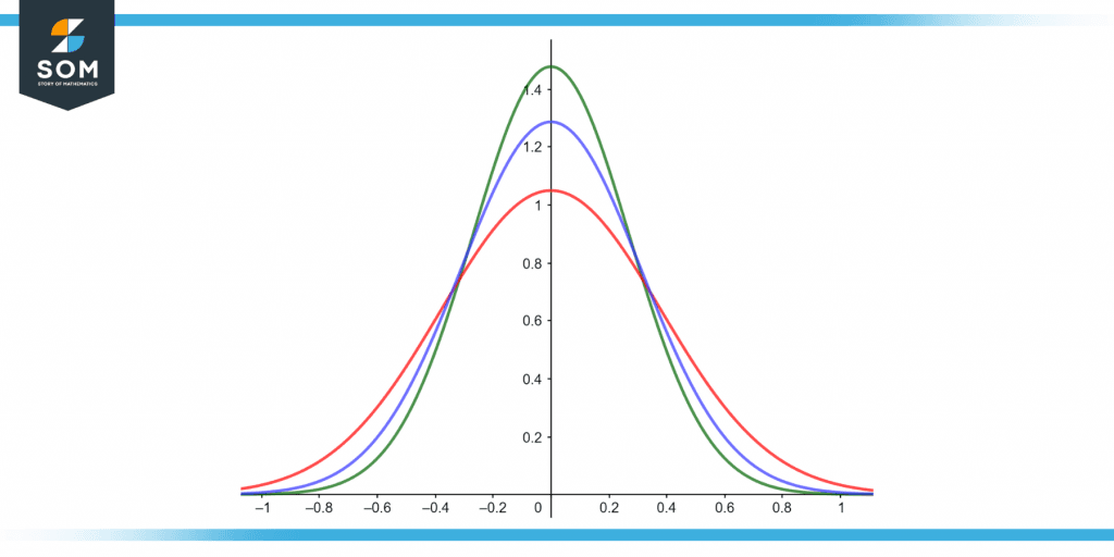
Figure 3 – Normal distribution with different sigma’s.

Examples of Normal Distribution

Below are some normal distribution examples that will help further clarify this topic.

Example 1

The average operating life of a particular brand for an electric light bulb is 1200 hours, with a standard variation of 200 hours. What is the likelihood of a bulb surviving longer than 1150 hours? Apply the normal distribution formula.

Solution

Let X, the working life, be distributed according to the normal distribution formula that follows:

X $\sim$ N(1200,$\mathsf{200^{2}}$)

Hence we get the following:

P(X > 1150) = 1 – P(X < 1150)

 Now by the formula, we get:

1 – $\mathsf{\varphi (\frac{1150-1200}{200})}$

Simplifying the equation: 1 – $\varphi$ (- 0.25)

So, the likelihood of a bulb surviving longer than 1150 hrs is 0.59871.

Example 2

Find the probability distribution function of the probability function if the stochastic process is 2, the mean is 5, and the standard deviation equals 4.

Solution

Given that x = 2 is a variable, 5 is the mean, and 4 is the standard deviation.

Using the probability distribution function of the normal distribution formula:

\[f(x,\mu ,\sigma )=\frac{1}{\sigma \sqrt{2\pi }^{e}}^{\frac{-(x-\mu)^{2}}{2\sigma^{2}}}\]

We may write:

\[f(2,2,4)=\frac{1}{4 \sqrt{2\pi }^{e}}^{\frac{-(2-2)^{2}}{(2)(4)^{2}}}\]

By solving, we get:

f(2,2,4) = 0.0997

All Images are made using GeoGebra.

Normal Definition < Glossary Index > Not Equal Definition