Tree|Definition & Meaning

A tree diagram is a tool used in probability and statistics in mathematics that enables us to count the number of possibilities that could occur in an event when those options are listed in an organised way. 

Each branch’s path in the tree diagram corresponds to a possible course for an event. It is an easy approach to depict the progression of events and it clearly and simply captures every conceivable result.

Tree diagrams often begin with a single item or node that branches into two or more, then each subsequent node will branch into two or more, and so on. The last diagram then looks like a tree with a trunk and several branches.

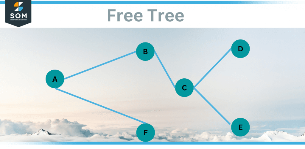
Figure 1 – A Free Tree diagram of 6 nodes

Usage of Tree in Probability

A tree diagram can be used to represent a probability space in probability theory. These diagrams could represent conditional probabilities or a series of separate events, like a set of coin tosses (like drawing cards from a deck, without substituting the cards).

Each node on the tree diagram represents an event and is linked to the likelihood that it will occur. Since the root node represents the particular event, its probability is 1. A comprehensive and independent spread of the parent event is shown by the entire collection of sibling joints or nodes.

When calculating probabilities, we occasionally run into problems and find it challenging to decide what to do.

The tree diagram will solve this problem. Think of a probability example to create a tree diagram for flipping a coin. Head and tail are the two branches. The outcome is placed at the branch’s end and the probability of an event is written on the branch.

Types of Trees

Free Trees

A connected graph with no cycles is all that a free tree is. There is just one method to get everywhere, and every node can be reached from every other node. It appears to be a graph, which it actually is, although it is less detailed than the WWII France graph. This is due to the fact that a free tree in certain ways doesn’t contain anything “additional.”

These fascinating facts are accurate if you have a free tree:

1. Any two nodes can only be reached by one path. (Verify it!)
2. The graph gets disconnected if any edge is removed. (Try it!)
3. Any additional edge results in the addition of a cycle. (Try it!)
4. There are n-1 edges when there are n nodes. (Consider it!)

In other words, if your objective is to link all the nodes and you have a free tree, you’re good to go. Anything you add is unnecessary, and anything you take away damages it.

This should bring to mind Prim’s algorithm, if not already. This is exactly what Prim’s algorithm produced: a free tree connecting all the nodes, and more specifically, the free tree with the least overall length.

A free tree that spans (connects) every node in the network is simply referred to as a “spanning tree.” Remember that the same set of vertices can be used to create a variety of free trees. For instance, you get a different free tree if you take away the edge from A to F and add one from anywhere else to F.

Decision Tree

Based on a hierarchical if-else classifier, a decision tree. The region is divided into a hypercube by the set of axis-parallel hyperplanes.

The decision tree uses a tree-like structure to construct classification or regression models. With an increase in tree depth, it divides a dataset into smaller subsets. The outcome is a tree containing leaf nodes and decision nodes.

Outlook is one example of a decision node that has two or more branches (e.g., Sunny, Overcast and Rainy). A classification or choice is represented by a leaf node (for instance, Play). The root node in a decision tree is the highest decision node that corresponds to the best predictor. Both category and numerical data can be processed using decision trees.

Rooted Tree

The only difference between a rooted tree and a free tree is that we elevate one node to serve as the root. It turns out that this is the deciding factor. Let’s say we determined that Figure 1’s root is A.

The rooted tree in Figure 2’s left half would then exist. Everything is flowing beneath the A vertex, which has been placed at the top. I picture it as delicately reaching into the free tree, gripping a node, and then lifting your hand up so the remaining nodes of the free tree dangle from it.

The right half of the illustration shows the rooted tree that would have resulted if we had instead picked (say) C as the root.The edges on both of these rooted trees are identical to those on the free tree: B is connected to both A and C, F is exclusively connected to A, etc. The root node’s designation is the only difference.

We have thus far stated that the spatial location on graphs is meaningless. But with rooted trees, this varies a little. We can only distinguish which nodes are “above” others through vertical orientation, and in this context, “above” refers to being nearer the root.

A node’s altitude indicates how many steps separate it from the root. Nodes B, D, and E are all one step away from the root (C) in the right rooted tree, whereas node F is three steps away.

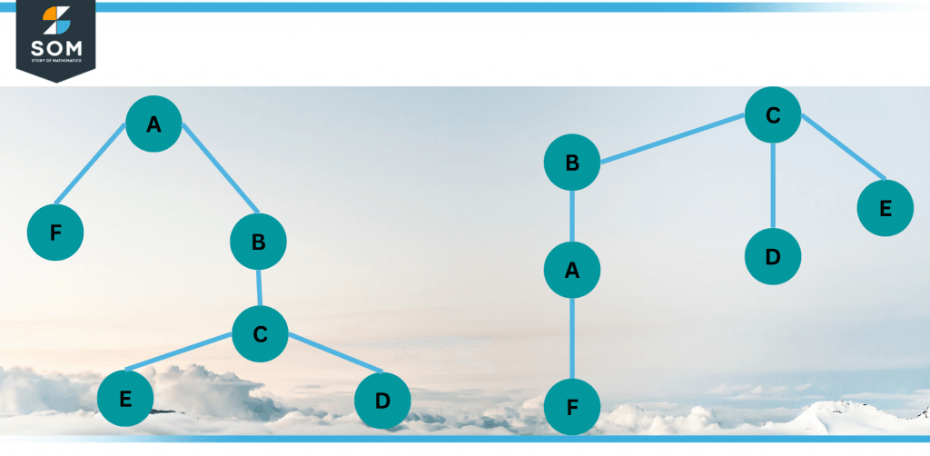
Figure 2 – Two distinct rooted trees with identical vertices and edges.

Binary Trees

A rooted tree’s nodes can have any number of offspring. However, there is a particular kind of rooted tree known as a binary tree that is constrained by merely stating that each node can have a maximum of two offspring. We’ll also refer to these two kids as the “left child” and “right child,” respectively. (Take note that a specific node may only have a left or right child, respectively, but it’s still crucial to know which way the kid is facing.)

Figure 2’s right half is not a binary tree, but its left half is (C has three children). Figure 3 displays a larger binary tree (of height 4).

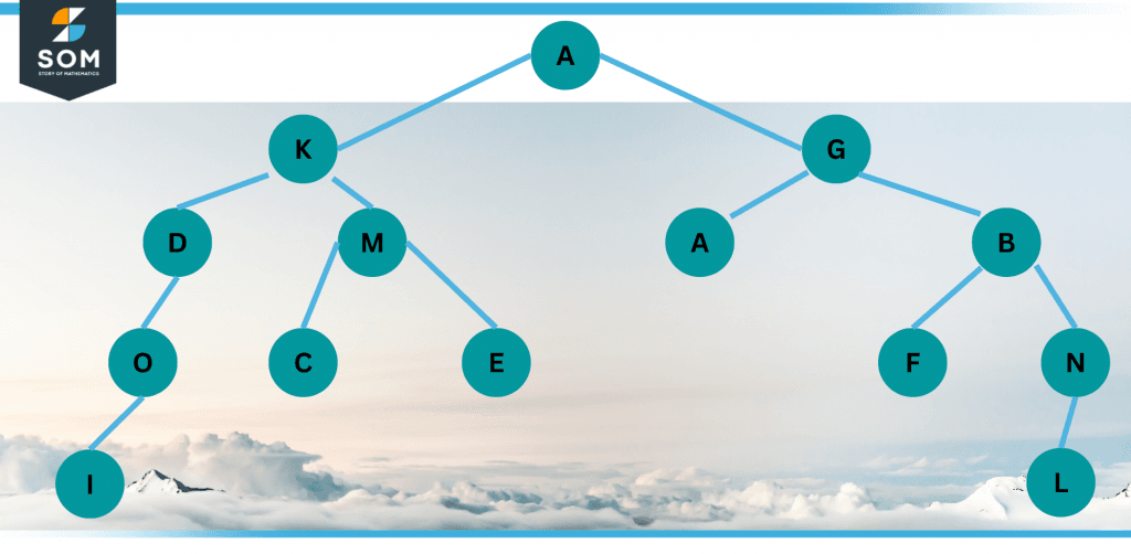
Figure 3 – A Binary Tree

Directed Trees

An acyclic-directed graph is a directed tree. It has one node with indegree 1 and all of the other nodes with indegree 1.
The node with outdegree 0 is known as an external node, a terminal node, or a leaf. Internal nodes are those with an outdegree greater than or equal to one.

Ordered Trees

A tree is referred to as being ordered if there is a definite ordering at each level of the tree.

Properties of Trees

• Because it has several levels, a tree is a hierarchical structure.
• The topmost node in a tree is referred to as the root node.
• A leaf node or terminal node is a node that is devoid of children.
• At every level of I 2i has the most nodes.
• The longest path from the root node to the leaf node is the height of the tree.
• The distance from a node’s root to the node’s depth.

Application of Trees

• In order to efficiently manage the data, trees hold data in the form of a hierarchical structure.
• Tree is also used to maintain the data in routing tables in the routers, which improves the insertion, deletion, and searching processes.

Example

Justify the fact that all trees are bipartite graphs.

Solution

The vertices of a graph must be split into two sets, A and B, such that no two vertices in either group are contiguous if we want to demonstrate that the graph is bipartite. This algorithm accomplishes exactly that.

Choose any vertex to serve as the root. Add this vertex to set A.

Place set B now to contain all of the root’s offspring. We are doing OK so far because none of these kids are close neighbors (they are all siblings). Put each child of each vertex in B into A now (i.e., every grandchild of the root). Alternate between A and B every “generation” until all vertices have been assigned to one of the sets. In other words, a vertex is only in set B if it is a child of a vertex in set.

All images/mathematical drawings were created with GeoGebra.

Trapezium Definition < Glossary Index > Trend Line Definition