JUMP TO TOPIC
Eigenvalue Calculator + Online Solver With Free Steps
An Eigenvalue Calculator is an online calculator that is used to find out the eigenvalues of an input matrix. These eigenvalues for a matrix describe the strength of the system of linear equations in the direction of a particular eigenvector.
Eigenvalues are used alongside their corresponding eigenvectors for analyzing matrix transformations as they tend to provide information about the matrix’s physical properties for real-world problems.

What Is a 2×2 Matrix Eigenvalue Calculator?
A 2×2 Matrix Eigenvalue Calculator is a tool that calculates eigenvalues for your problems involving matrices and is an easy way of solving eigenvalue problems for a 2×2 matrix online.
It solves the system of linear equations in your browser and gives you a step-by-step solution. The eigenvalues and their eigenvectors for these input matrices, therefore, have a massive significance. These provide a strong correlation between the system of linear equations and their validity in the real world.
Eigenvalues and eigenvectors are well-known
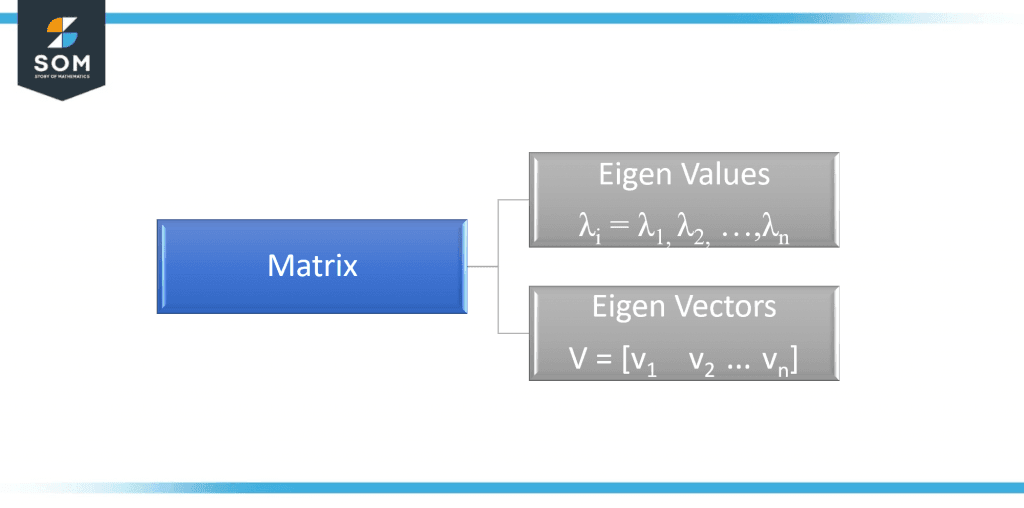
Figure-1 Eigen values and eigen vectors
in the field of mathematics, physics, and engineering. This is because these values and vectors help in describing a lot of complex systems.
They are used most commonly to identify directions and magnitudes for stresses acting on irregular and complex geometries. Such work relates to the field of mechanical and civil engineering. The calculator is designed to get the entries of a matrix and provides the appropriate results after running its calculations.
The Eigenvalue Calculator has input boxes for each entry of the matrix, and it can provide you with the desired results at the touch of a button.
How To Use the Eigenvalue Calculator 2×2?
This Eigenvalue Calculator is very easy and intuitive to use, with only four input boxes and a “Submit” button. It is important to note that it can only work for 2×2 matrices and not for any order above that, but it is still a useful tool for quickly solving your eigenvalue problems.
The guidelines for using this calculator to get the best results are as follows:
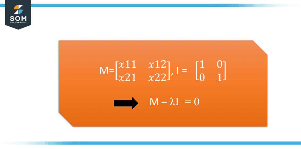
Figure-2 Steps to find Eigen Values
Step 1:
Take a matrix problem that you would like to solve the eigenvalues for.
Step 2:
Enter the values of your 2×2 matrix problem into the 4 input boxes available at the calculator’s interface.
Step 3:
Once the entry is done, all you need to do is to press the “Submit” button and the solution will appear in a new window.
Step 4:
Finally, to view the step-by-step solution to the problem, you can click the appropriate button provided. If you intend to solve another problem, you can easily do that as well by entering the new values in the open window.
How Does a 2×2 Matrix Eigenvalue Calculator Work?
This Eigenvalue calculator works by using matrix addition and multiplication at its core for finding the required solution. Let’s discuss how an Eigenvalue Calculator works.
What Is an Eigenvalue?
An eigenvalue is a value that represents several scalar quantities that correspond to a system of linear equations. This value for a matrix gives information regarding its physical nature and quantity. This physical quantity is handled in the form of magnitude, acting in a particular direction which is described by the eigenvectors for the given matrix.
These values are referred to by a lot of different names in the world of mathematics i.e., characteristic values, roots, latent roots, etc. but they are most commonly known as Eigenvalues around the world.
Setup the Input in the Desired Form:
Having a huge significance in the world of physics, mathematics, and engineering, eigenvalues are one important set of quantities. Now, this Eigenvalue calculator uses matrix addition and multiplication at its core for finding the required solution.
We start by assuming that there is a matrix A which is given to you with an order of n x n. In the case of our calculator, to be specific this matrix must be of the order 2 x 2. Now let there be a set of scalar values associated with this matrix described by Lambda ( $\lambda$). The relationship between the scalar ( $\lambda $) with the input matrix A is provided to us as follows:
|A – $\lambda$ . I| = 0
Solve for the New Form To Get the Result:
Where A represents the input matrix of the order 2×2, I represents the identity matrix of the same order, and \lambda is in there representing a vector that contains the eigenvalues associated with the matrix A. Thus, $\lambda$ is also known as the Eigen matrix or even the characteristic matrix.
Finally, the vertical bars on each side of this equation show that there is a determinant acting on this matrix. This determinant will then be equated to zero under the given circumstances. This is done to calculate the appropriate latent roots, which we refer to as eigenvalues of the system.
Therefore, a matrix A will have a corresponding set of eigenvalues $\lambda$ when |A – $\lambda$ . I| = 0.
Steps for Finding Out a Set of Eigenvalues:
- Let’s assume that there is a square matrix namely A with an order of 2×2, where the identity matrix is expressed as \begin{pmatrix} 1 & 0 \\ 0 & 1 \end{pmatrix}
- Now, to get the desired equation, we must introduce a scalar quantity i.e., \lambda that shall be multiplied by the identity matrix I.
- Once this multiplication is completed, the resultant matrix is subtracted from the original square matrix A, (A – $\lambda$ . I).
- Finally, we calculate the resulting matrix’s determinant, |A – $\lambda$ . I|.
- The result, when equated to zero, |A – $\lambda$ . I| = 0 ends up making a quadratic equation.
- This quadratic equation can be solved to find the eigenvalues of the desired square matrix A of order 2×2.
Relationship Between Matrix and Characteristic Equation:
One important phenomenon to note is that, for a 2×2 matrix, we will get a quadratic equation and two eigenvalues, which are the roots extracted from that equation.
Therefore, if you identify the trend here, it becomes apparent that as the order of the matrix increases, so does the degree of the resulting equation and eventually the number of roots it produces.
History of Eigenvalues and Their Eigenvectors:
Eigenvalues have been commonly used alongside systems of linear equations, matrices, and linear algebra problems in the modern day. But originally, their history is tied more closely with the differential and quadratic forms of equations than the linear transformation of matrices.
Through the study brought forth by the 18th-century mathematician Leonhard Euler, he was able to discover the true nature of a rigid body’s rotational motion, that the principal axis of this rotating body was the inertia matrix’s eigenvectors.
This led to a massive breakthrough in the field of mathematics. In the early 19th century, Augustin-Louis Cauchy found a way to describe quadratic surfaces numerically. Once generalized, he had found the characteristic roots of the characteristic equation, now commonly known as Eigenvalues, and that lives on to this day.
Solved Examples:
Example No.1
Consider the following system of linear equations and solve for its corresponding eigenvalues:
\[ A = \begin{bmatrix}
0 & 1 \\
-2 & -3
\end{bmatrix} \]
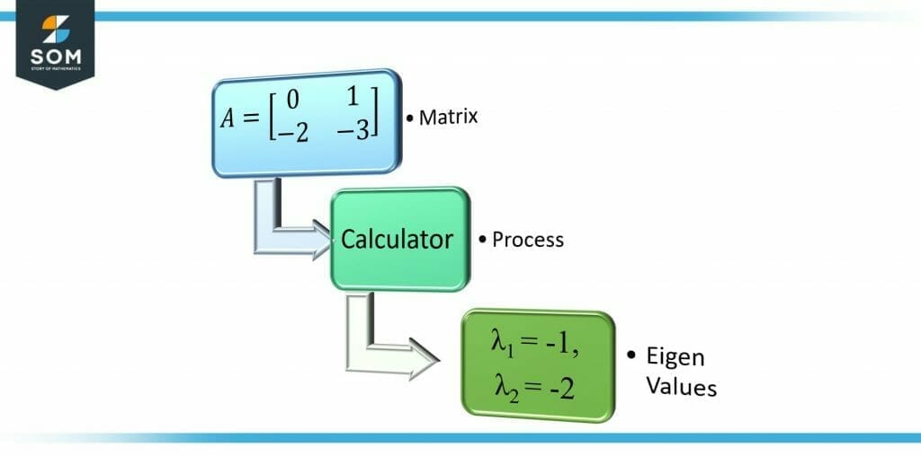
Figure-3 Solved Example
Now the given matrix can be expressed in the form of its characteristic equation as follows:
\[ |A – \lambda \cdot I| =\bigg|\begin{bmatrix}
0 & 1 \\
-2 & -3
\end{bmatrix} – \begin{bmatrix}\lambda & 0 \\0 & \lambda \end{bmatrix}\bigg| = 0\]
Solving this matrix further produces the following quadratic equation:
\[\bigg|\begin{bmatrix}-\lambda & 1 \\-2 & -3-\lambda \end{bmatrix}\bigg| = \lambda^2 + 3\lambda + 2 = 0\]
Finally, the solution to this quadratic equation leads to a set of roots. These are the associated eigenvalues to the system of linear equations given to us:
$\lambda$1 = -1, $\lambda$2 = -2
Example No.2
Consider the following system of linear equations and solve for its corresponding eigenvalues:
\[ A = \begin{bmatrix}
-5 & 2 \\
-9 & 6
\end{bmatrix} \]
Now the given matrix can be expressed in the form of its characteristic equation as follows:
\[|A – \lambda \cdot I|=\bigg|\begin{bmatrix}
-5 & 2 \\
-9 & 6
\end{bmatrix} – \begin{bmatrix}\lambda & 0 \\0 & \lambda \end{bmatrix}\bigg| = 0\]
Solving this matrix further produces the following quadratic equation:
\[\bigg|\begin{bmatrix}-5-\lambda & 2 \\-9 & 6-\lambda \end{bmatrix}\bigg| = \lambda^2 – \lambda – 12 = 0\]
Finally, the solution to this quadratic equation leads to a set of roots. These are the associated eigenvalues to the system of linear equations given to us:
$\lambda$1 = -3, $\lambda$2 = 4
Example No.3
Consider the following system of linear equations and solve for its corresponding eigenvalues:
\[A =\begin{bmatrix}2 & 3 \\2 & 1\end{bmatrix}\]
Now the given matrix can be expressed in the form of its characteristic equation as follows:
\[|A – \lambda \cdot I| = \bigg|\begin{bmatrix}2 & 3 \\2 & 1 \end{bmatrix} – \begin{bmatrix}\lambda & 0 \\0 & \lambda \end{bmatrix}\bigg| = 0\]
Solving this matrix further produces the following quadratic equation:
\[\bigg|\begin{bmatrix}2-\lambda & 3 \\2 & 1-\lambda \end{bmatrix}\bigg| = \lambda^2 – 3 \lambda – 4 = 0\]
Finally, the solution to this quadratic equation leads to a set of roots. These are the associated eigenvalues to the system of linear equations given to us:
$\lambda$1 = 4, $\lambda$2 = -1
Example No.4
Consider the following system of linear equations and solve for its corresponding eigenvalues:
\[A =\begin{bmatrix}5 & 4 \\3 & 2\end{bmatrix}\]
Now the given matrix can be expressed in the form of its characteristic equation as follows:
\[|A – \lambda \cdot I| = \bigg|\begin{bmatrix}5 & 4 \\3 & 2 \end{bmatrix} – \begin{bmatrix}\lambda & 0 \\0 & \lambda \end{bmatrix}\bigg| = 0\]
Solving this matrix further produces the following quadratic equation:
\[\bigg|\begin{bmatrix}5-\lambda & 4 \\3 & 2-\lambda \end{bmatrix}\bigg| = \lambda^2 – 7 \lambda – 2 = 0\]
Finally, the solution to this quadratic equation leads to a set of roots. These are the associated eigenvalues to the system of linear equations given to us:
$\lambda$1 = 4, $\lambda$2 = 3