General Solution Calculator + Online Solver With Free Steps

The online General Solution Calculator is a calculator that allows you to find the derivatives for a differential equation.

The General Solution Calculator is a fantastic tool that scientists and mathematicians use to derive a differential equation. The General Solution Calculator plays an essential role in helping solve complex differential equations.

What Is a General Solution Calculator?

A General Solution Calculator is an online calculator that helps you solve complex differential equations. 

The General Solution Calculator needs a single input, a differential equation you provide to the calculator. The input equation can either be a first or second-order differential equation. The General Solution Calculator quickly calculates the results and displays them in a separate window.

The General Solution Calculator displays several different results such as the input, the plots of the equation, alternative form, complex roots, polynomial discriminant, the derivative, the integral, and global minimum if available.

How To Use a General Solution Calculator?

You can use the General Solution Calculator by entering the differential equation in the calculator and clicking the “Submit” button on the General Solution Calculator. 

The step-by-step instructions on how to use a General Solution Calculator are given below:

Step 1

To use the General Solution Calculator, you must first plug your differential equation in its respective box.

Step 2

Once you have entered the differential equation in the General Solution Calculator, you simply click the “Submit” button. The General Solution Calculator will perform the calculations and instantly display the results on a new window.

How Does a General Solution Calculator Work?

A General Solution Calculator works by taking a differential equation as an input represented as y = f(x) and calculating the results of the differential equation. Solving a differential equation gives us insight into how quantities change and why this change occurs.

What Are Differential Equations?

A differential equation is an equation that contains the derivative of an unknown function. The derivatives of a function determine how quickly it changes at a given point. These derivatives are connected to the other functions using a differential equation. 

The principal applications of differential equations are used in the sciences of biology, physics, engineering, and many more. The differential equation’s primary goal is to study the solutions that satisfy the equations and the solutions’ characteristics.

Any equation with at least one ordinary or partial derivative of an unknown function is referred to as a differential equation. Assuming that a function’s rate of change about x is inversely proportional to y, we may write it down as $\frac{dy}{dx} = \frac{k}{y}$.

A differential equation in calculus is an equation that involves the dependent variable’s derivatives concerning the independent variable. The derivative is nothing more than a representation of the rate of change. 

The differential equation aids in presenting a relationship between the changing quantity and the change in another quantity. Let y=f(x) be a function, where f is an unknown function, x is an independent variable, and f is the dependent variable.

What Are Order of Differential Equations?

The order of a differential equation is the order that is determined by the highest order derivative that appears in the equation. Consider the following differential equations:

\[ \frac{dx}{dy} = e^{x} , (\frac{d^{4}x}{dy^{4}}) + y = 0 , (\frac{d^{3}x}{dy^{3}}) + x^{2}(\frac{d^{2}x}{dy^{2}}) = 0 \]

The highest derivatives in the examples of differential equations above are first, fourth, and third-order, respectively.

First Order of Differential Equations

The first example demonstrates a first-order differential equation with a degree of 1. The first order includes all linear equations that take the form of derivatives. It only has the first derivative, as shown by the equation $\frac{dy}{dx}$, where x and y are the two variables, and $\frac{dy}{dx} = f(x, y) = y’$.

Second-Order of Differential Equations

The second-order differential equation is the equation that contains the second-order derivative. Second-order derivates are represented by this equation $\frac{d}{dx}(\frac{dy}{dx}) = \frac{d^{2}y}{dx^{2}} = f”(x) = y” $.

What Are Ordinary Differential Equations?

An ordinary differential equation or ODE is a mathematical equation with only one independent variable and one or more of its derivatives. 

As a result, the ordinary differential equation is represented as a relationship between the real dependent variable y and one independent variable x, together with some of y’s derivatives about x. 

Since the differential equation in the example below lacks partial derivatives, it is an ordinary differential equation.

\[ (\frac{d^{2}y}{dx^{2}})+(\frac{dy}{dx})=3y\cos{x} \]

There are two types of homogeneous and non-homogeneous ordinary differential equations.

What Are Homogeneous Differential Equations?

Homogenous differential equations are differential equations in which all terms have the same degree. Since P(x,y) and Q(x,y) are homogeneous functions of the same degree, they can be generally expressed as P(x,y)dx + Q(x,y)dy = 0.

Here are some examples of homogeneous equations:

\[ y + x(\frac{dy}{dx}) = \text{0 is a homogeneous differential equation of degree 1} \]

\[ x^{4} + y^{4}(\frac{dy}{dx}) = \text{0 is a homogeneous differential equation of degree 4} \]

What Are Non-homogeneous Differential Equations?

A non-homogenous differential equation is an equation in which each term’s degree is different from the others. The equation $xy(\frac{dy}{dx}) + y^{2} + 2x = 0$ is an example of non-homogenous differential equation.

The linear differential equation is a kind of non-homogenous differential equation and is related to the linear equation.

What Are Partial Differential Equations?

A partial differential equation, or PDE, is an equation that only uses the partial derivatives of one or more functions of two or more independent variables. The following equations are examples of partial differential equations:

\[ \frac{\delta{u} }{dx} + \frac{\delta}{dy} = 0 \]

\[ \frac{\delta ^{2}u}{\delta x^{2}} + \frac{\delta ^{2}u}{\delta x^{2}} = 0 \]

Applications of Differential Equations

Ordinary differential equations are used in everyday life to compute the flow of electricity, the motion of an object back and forth like a pendulum, and to illustrate the principles of thermodynamics.

In medical terminology, they are also used to monitor disease progression graphically. Mathematical models involving population increase or radioactive decay can be described using differential equations.

Solved Examples

The General Solution Calculator is a quick and easy way to calculate a differential equation.

Here are some examples solved using the General Solution Calculator:

Solved Example 1

A college student is presented with an equation $ y = x^{3} + x^{2} + 3 $. He needs to calculate the derivative of this equation. Using the General Solution Calculator, find the derivative of this equation.

Solution

Using our General Solution Calculator, we can easily find the derivative for the equation given. First, we add the equation to its respective box in the calculator. 

After entering the equation, we click the “Submit” button. The General Solution Calculator quickly computes the equation and displays the results in a new window.

The results from the General Solution Calculator are shown below:

Inputs:

\[ y = x^{3} + x^{2} + 3 \]

Plot:

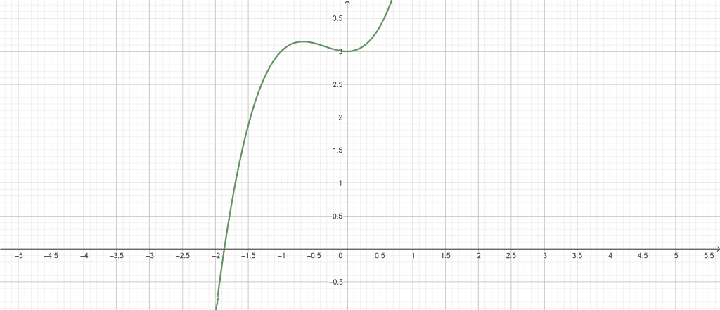
Figure 1

Alternate Form:

\[ – x^{3} – x^{2} – 3 = 0 \]

Real Root:

x $\approx$ -1.8637 

Complex Roots:

x $\approx$ 0.43185 – 1.19290i 

 x $\approx$ 0.43185 + 1.19290i 

Partial Derivatives:

\[ \frac{\partial}{\partial x} (x^{3} + x^{2} + 3) = x(3x+2) \]

\[ \frac{\partial}{\partial y} (x^{3} + x^{2} + 3) = 0 \]

Implicit Derivative:

\[ \frac{\partial x(y)}{\partial y} = \frac{1}{2x+3x^{2}} \]

\[ \frac{\partial y(x)}{\partial x} = x(2 + 3x) \]

Local Maxima:

\[ max\left \{ x^{3} + x^{2} + 3 \right \} = \frac{85}{27} \ at \ x=-\frac{2}{3} \]

Local Minima:

\[ max\left \{ x^{3} + x^{2} + 3 \right \} = 3 \ at \ x= 0 \]

Solved Example 2

While researching a scientist comes across the following equation:

\[ y =  x^{3} +5x^{2}  + 3x \]

To continue his research, the scientist needs to determine the derivative of the equation. Find the derivative of the equation provided.

Solution

We can solve the equation by using the General Solution Calculator. Initially, we input the equation provided to us in the calculator. 

Once we enter the equation in the General Solution Calculator, we all need to click the “Submit” button. The calculator will instantly display the results in a new window.

The results from the General Solution Calculator are shown below:

Input:

\[ y =  x^{3} +5x^{2}  + 3x \]

Plot:

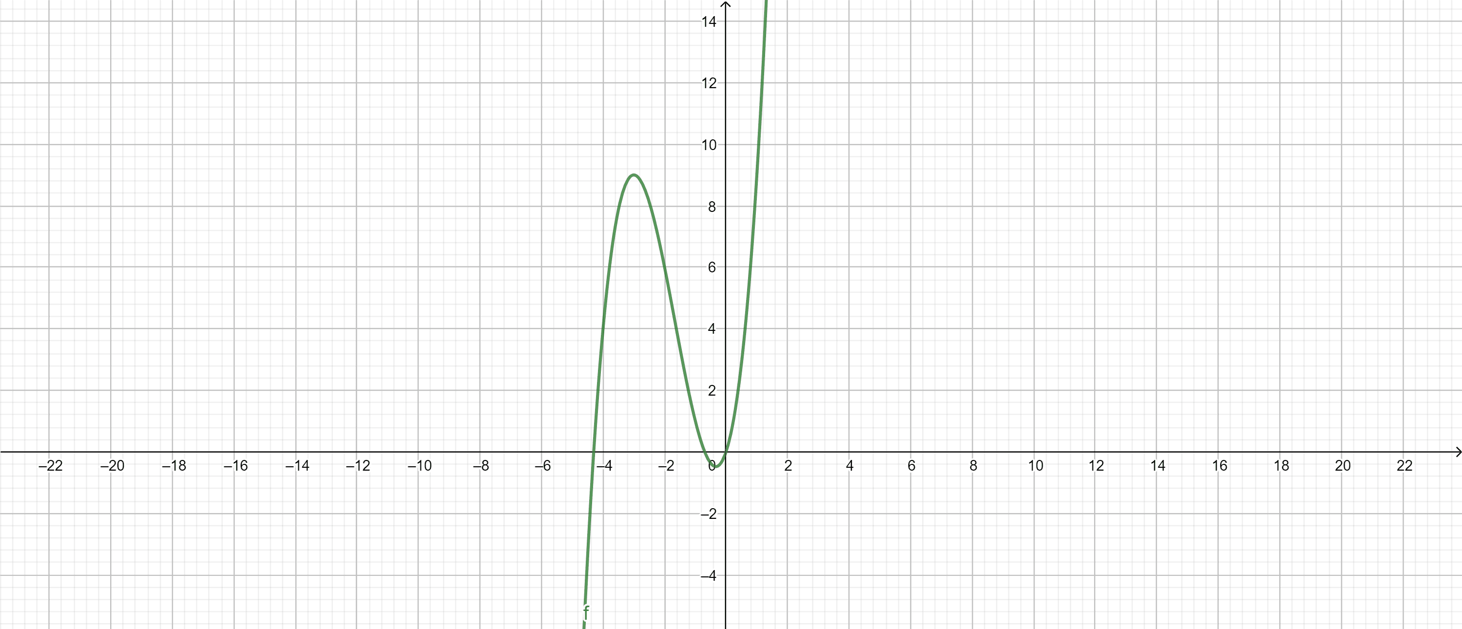
Figure 2

Alternate Form:

y = x(x(x+5)+3) 

\[ y = x(x^{2} + 5x + 3) \]

\[ -x^{3} – 5x^{2}  – 3x = 0 \]

Roots:

x = 0 

\[ x = -\frac{5}{2}-\frac{\sqrt{13}}{2} \]

\[ x=  \frac{\sqrt{13}}{2} – \frac{5}{2} \]

Domain:

\[ \mathbb{R} \ (all \ real \ numbers ) \]

Range:

\[ \mathbb{R} \ (all \ real \ numbers ) \]

Surjectivity:

\[ Surjectivity \ onto \ \mathbb{R} \]

Partial Derivatives:

\[ \frac{\partial }{\partial x}( x^{3} +5x^{2}  + 3x) = 3x^{2} + 10x + 3 \]

\[ \frac{\partial }{\partial y}( x^{3} +5x^{2}  + 3x) = 0 \]

Implicit Derivative:

\[ \frac{\partial x(y)}{\partial y} = \frac{1}{3+10x+3x^{2}} \]

\[ \frac{\partial y(x)}{\partial x} = 3+10x+3x^{2} \] 

Local Maxima:

\[ max\left \{ x^{3} +5x^{2}  + 3x \right \} = 9 \ at \ x = -3 \]

Local Minima:

\[ max\left \{ x^{3} +5x^{2}  + 3x \right \} = -\frac{13}{27} \ at \ x = -\frac{1}{3} \]

All images/graphs are created using GeoGebra

Sequence Formula Calculator < Math Calculators List > Arc Length Calculator Calculus